0060 MonetDB – Data Types
Strings
All CHARACTER data types are using UTF-8.
| Name | Aliases | Description |
| CHARACTER | CHARACTER(1), CHAR, CHAR(1) | 0 or 1 character |
| CHARACTER (length) | CHAR(length) | Fixed length. String is returned without padding spaces, but it is stored with padding spaces. |
| CHARACTER VARYING (length) | VARCHAR (length) | "Length" is a maximal number of characters for this string. |
| CHARACTER LARGE OBJECT | CLOB, TEXT, STRING | String of unbounded length. |
| CHARACTER LARGE OBJECT (length) | CLOB (length), TEXT (length), STRING (length) | String with maximal number of characters. CLOB(N) is similar to VARCHAR(N), but it can hold much bigger string, although it seems that in MonetDB there is no difference between them. |
Binary objects
| Name | Aliases | Description |
| BINARY LARGE OBJECT | BLOB | Binary objects with unbounded length. |
| BINARY LARGE OBJECT ( length ) | BLOB ( length ) | Binary objects with maximal length. |
Numbers
Boolean data type can be considered as 0 or 1. So, all data types below are for numbers. "Prec(ision)" is total number of digits. "Scale" are digits used for decimals. For number 385,26; "Prec" is 5 (3+2), and "Scale" is 2. For all number data types, precision is smaller than 18 (or 38 on linux).
| Name | Aliases | Description |
| BOOLEAN | BOOL | True of False. |
| TINYINT | Integer between -127 and 127 (8 bit) | |
| SMALLINT | Integer between -32767 and 32767 (16 bit) | |
| INTEGER | INT, MEDIUMINT | Integer between -2.147.483.647 and 2.147.483.647 (32 bit) |
| BIGINT | 64 bit signed integer | |
| HUGEINT | 128 bit signed integer | |
| DECIMAL | DEC, NUMERIC | Decimal number, where "Prec" is 18, and "Scale" is 3. |
| DECIMAL ( Prec ) | DEC ( Prec ), NUMERIC ( Prec ) | Zero decimals, but we decide on total number of digits ("Prec"). |
| DECIMAL ( Prec , Scale ) | DEC ( Prec , Scale ), NUMERIC ( Prec , Scale ) | We decide on "Prec(ision)" and "Scale". |
| REAL | FLOAT(24) | 32 bit approximate number. |
| DOUBLE PRECISION | DOUBLE, FLOAT, FLOAT(53) | 64 bit approximate number. |
| FLOAT ( Prec ) | FLOAT(24) is same as REAL, FLOAT(53) is same as DOUBLE PRECISION. In this case precision can be only between 1 and 53 because this is special kind of precision ( binary (radix 2) precision ). |
Time
These are time data types. "Prec(ision)" now has different meaning. "Prec" is number of digits used for fraction of a second. For 33,7521 seconds, "Prec" is 4. In all cases below, "Prec" has to be between 0 and 6.
| Name | Aliases | Description |
| DATE | Date YYYY-MM-DD. | |
| TIME | TIME(0) | Time of day HH:MI:SS. |
| TIME ( Prec ) | TIME with fraction of a second (HH:MI:SS.ssssss). | |
| TIME WITH TIME ZONE | TIME(0) WITH TIME ZONE | TIME of day with a timezone (HH:MI:SS+HH:MI). |
| TIME ( Prec ) WITH TIME ZONE | Same as above, but now with fraction of a second (HH:MI:SS.ssssss+HH:MI). | |
| TIMESTAMP | TIMESTAMP(6) | Combination of a DATE and TIME(6) (YYYY-MM-DD HH:MI:SS.ssssss). |
| TIMESTAMP ( Prec ) | Same as above, but we decide on "Prec(ision)". | |
| TIMESTAMP WITH TIME ZONE | TIMESTAMP(6) WITH TIME ZONE | TIMESTAMP(6) with a timezone (YYYY-MM-DD HH:MI:SS.ssssss+HH:MI). |
| TIMESTAMP ( Prec ) WITH TIME ZONE | Same as above, but we decide on "Prec(ision)". |
INTERVAL
Interval is the difference between two dates and times. There are two measure units to express interval. One is to use number of months. The other is time interval that is expressed in seconds with milliseconds precision. These two types can not be mixed because months have varying numbers of days.
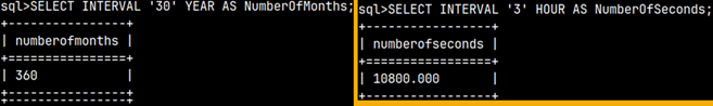
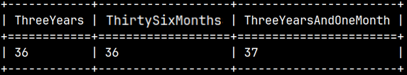
There are three data types if you are using number of months: YEAR, MONTH and YEAR TO MONTH.
SELECT INTERVAL '3' YEAR AS "ThreeYears"
     , INTERVAL '36' MONTH AS "ThirtySixMonths"
     , INTERVAL '0003-01-01' YEAR TO MONTH AS "ThreeYearsAndOneMonth";
If you are using seconds as measurement unit then we have 10 data types:
| INTERVAL DAY | INTERVAL DAY TO HOUR | INTERVAL DAY TO MINUTE | INTERVAL DAY TO SECOND | INTERVAL HOUR |
| INTERVAL HOUR TO MINUTE | INTERVAL HOUR TO SECOND | INTERVAL MINUTE | INTERVAL MINUTE TO SECOND | INTERVAL SECOND |
SELECT INTERVAL '1' DAY AS "Day"                                                   --1*24*60*60
            , INTERVAL '1 01' DAY TO HOUR AS "DayToHour"                           --DAY+60*60
            , INTERVAL '1 01:01' DAY TO MINUTE AS "DayToMinute"                    --DAY+60*60+60
            , INTERVAL '1 01:01:01.333' DAY TO SECOND AS "DayToSecond"             --DAY+60*60+60+1,333
            , INTERVAL '1' HOUR AS "Hour"                                          --60*60
            , INTERVAL '01:01' HOUR TO MINUTE AS "HourToMinute"                    --HOUR+60
            , INTERVAL '01:01:01.333' HOUR TO SECOND AS "HourToSecond"             --HOUR+60+1,333
            , INTERVAL '1' MINUTE AS "Minute"                                      --60
            , INTERVAL '01:01.333' MINUTE TO SECOND AS "MinuteToSecond"            --60+1,333
            , INTERVAL '15.333' SECOND AS "Second"                                 --15,333
            ;
| For seconds data type, maximal precision is up to milliseconds. Result is always expressed with three decimals. | 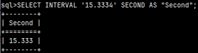 |
| For "YEAR TO MONTH" we can also write "SELECT INTERVAL '2-5' YEAR TO MONTH". | 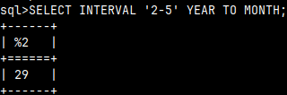 |
TIME ZONES
Timestamp is combination of date and time. Timestamp time is time without daylight savings time (DST) regime. This time should represent Greenwich time.
For getting correct time, we should provide time zone with each database connection so that Greenwich time is transformed to local time. Timestamps '15:16:55+02:00' and '14:16:55+01:00' are presenting the same time but for users in different time zones. Timestamp '15:16:55+02:00' and '14:16:55+01:00' are both presenting Greenwich time of '13:16:55+00:00' because 15 – 2=13 and 14 – 1= 13.
If we want, we can change our connection time zone setting by issuing statement "SET TIME ZONE INTERVAL '01:00' HOUR TO MINUTE". This statement "SELECT CURRENT_TIMEZONE" would tell us what is our current time zone. | 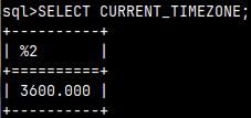 |
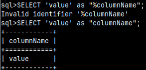 SELECT 'value' as "columnName";
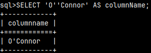


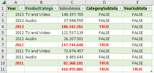
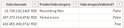
 this is filter table created with TREATAS function.