In the internet browser we can observe certificate of some web site. First, we click on the padlock in the address bar (1). We click on "Connection is secure" (2). Then we click on the icon (3). After that a new dialog with a certificate will open (4). We can also observe certificate with OpenSSL. OpenSSL has command "s_client" that is used to test and monitor TLS connection. When we use this command, terminal will enter interactive mode where we can type HTTP, SMTP, POP3, LDAP commands. This assumes that "s_client" is connected to some server application and can now communicate with that application using its protocol. For example, SMTP is computer protocol used for sending emails. We are not going to use this client in interactive mode in this article. We will use it only to observe TLS information.

Certificate

S_client Interactive Mode

This command will connect OpenSSL to web site as a TLS client. openssl s_client -connect www.example.com:443   As a result, we would get a lot of text, and after that text we will get a prompt. Prompt means that we are in the interactive mode.
	I will click "Ctrl+C" to exit this prompt.
"/dev/null" is a feature of terminal. This means that s_client will not receive commands from a keyboard, but from a file. File "/dev/null" is empty file. This will send EOF ( end of file ) signal to s_client and s_client will immediately exit interactive mode. I will use this to avoid interactive mode. openssl s_client -connect www.example.com:443 </dev/null

Reading the Certificate with S_client

OpenSSL command "x509" is for working with certificates. Text returned by the "-connect" command can be piped to "openssl x509" command.

openssl s_client -connect example.com:443 </dev/null | openssl x509

Certificate will be returned in PEM format. This is base64 encoded format. This format prints each 6-bits with a printable character.

We want nicely presented text, like on the image to the right. To get this text we have to use "-text" option.

Without options we have PEM format. With "-text" option we have PEM, and human readable format. With "-text" and "-noout" we only get human readable format.

So, the full command will be like this. "-text" will give us nicely formatted certificate, and "-noout" will suppress PEM format.

openssl s_client -connect example.com:443 </dev/null | openssl x509 -text -noout

Main Sections of a Certificate

Certificate is divided into 3 sections.

– Data: This is certificate in a readable form. – Signature Algorithm: This algorithm CA used to sign the certificate. – Signature Value: This is certificate signed ( encrypted ). CA used "Signature Algorithm" to encrypt "Data" and the result is "Signature Value". Here we have all of the elements to identify the owner and to verify his identity.

Data part is mostly hidden on the image above, but that is the biggest part of the certificate. It contains info about CA and certificate owner, data about certificate itself, and the public key of the certificate owner.

Data Section Content

Version – there are several generations of certificates specification. Today we use version 3. Serial Number – our CA is using this number to distinguish our certificate from other certificates issued by the same CA. Signature Algorithm – CA used ECDSA asymmetric key to sign our certificate. Issuer – Data about CA. We can see the country ( "C" ), organization legal name ( "O" ), common name ( "CN" ). "CN" is for less formal name of the organization. Validity – Period in which our certificate is valid. Subject – this is where we place the name of domain ( example.com ). Subject Public Key Info – data about certificate owner public key. Here we can see algorithm, the size of a key and the key itself.

Below this we have extensions. Extensions are specialized elements and we will talk about in some other article.

Reading Only Some Sections of a Certificate

We can limit our command to read only some elements.

openssl s_client -connect example.com:443 </dev/null \        | openssl x509 -noout -serial -issuer -subject -pubkey
openssl s_client -connect example.com:443 </dev/null \        | openssl x509 -noout -dates

S_client

ServerName Option

Cloud providers can host several web sites behind one IP address. Each of those sites can have its separate certificate. Cloud provider must know in advance what certificate to send to the user.   This is why for s_client we must use option "-servername".   openssl s_client -connect www.google.com:443 -servername maps.google.com

Look below how we are getting different answer depending on the servername we use.

openssl s_client -connect www.google.com:443 -servername maps.google.com </dev/null | openssl x509 -noout -subject >>>>>              subject=CN = *.google.com              <<<<<

openssl s_client -connect www.google.com:443 -servername www.google.com </dev/null | openssl x509 -noout -subject >>>>>              subject=CN = www.google.com              <<<<<

Quiet and Brief Options

With "-quiet" option we will start interactive mode, without getting certificate. openssl s_client -connect www.example.com:443 -quiet
"-brief" option is similar, but we are still getting some essential data.   openssl s_client -connect www.example.com:443 -brief

"-Brief" allow us to see what cipher suite and protocol version the client and the server made an agreement to use ( TLSv1.3: TLS_AES_256_GCM_SHA384 ).

Protocol and Cipher Suite Options

We can force the protocol s_client will use. openssl s_client -connect www.example.com:443 -brief -tls1_2
We can enforce specific cipher suite. openssl s_client -connect www.example.com:443 -brief -tls1_2 -cipher AES256-SHA256
We can block protocol TLSv1.3. openssl s_client -connect www.example.com:443 -brief -no_tls1_3

Certopt Option

We already saw that certificate includes public key of the certificate owner, and it has sections Signature Algorithm and Signature Value. We can use option "-certop" to suppress those elements. We can suppress both elements or only one of them.

openssl s_client -connect www.mwl.io:443  < /dev/null | openssl x509 -text -noout -certopt no_pubkey,no_sigdump

This part will be missing because of "no_pubkey".

"no_sigdump" will make two last sections to be excluded.

Certificate Chains

In our browser we will take a look at certificate for the web site "www.example.com". In the "details" tab we can see so-called "certificate chain". Chain certificate means that sometimes we need more certificates to prove that the certificate we own is valid. These certificates are connected in a hierarchy with root certificate at the top ( CA certificate ), and leaf certificate at the bottom ( example.com ). Between them we can have several intermediate certificates.

If we want to read all of these certificates we need "-showcerts" option. openssl s_client -connect www.example.com:443 -servername www.example.com -showcerts      We will get 4 "BEGIN/END CERTIFICATE" elements =>

Certificate chain can not be presented in nice readable form with the use of "x509" command, only in PEM format.

Certificate Export

The whole chain of certificates can be exported to a file with simple redirection. openssl s_client-connect www.example.com:443 -showcerts < /dev/null > /home/fff/Desktop/certificates.chain
We can save leaf certificate nicely formatted with "-out" option. openssl s_client -connect www.example.com:443 < /dev/null | openssl x509 -text -out /home/fff/Desktop/certificate.crt
We saw that our certificate can be in the PEM format. There are other formats, like DER format which is a binary form of format. We can specify in which format to export certificate with "-outform" option. openssl s_client -connect www.example.com:443 </dev/null | openssl x509 -outform PEM -out /home/fff/Desktop/PEM.crt openssl s_client -connect www.example.com:443 </dev/null | openssl x509 -outform DER -out /home/fff/Desktop/DER.crt

Errors

We can test TLS errors on the web site "www.badssl.com". Option "-verify return error" will suppress showing of the certificate and will return much smaller message where we can easily notice what is the problem with the certificate.

openssl s_client -connect expired.badssl.com:443 -verify_return_error

Hostname Verification

If we go to a website ( x.com ) and download its certificate, but inside the certificate we see another domain ( y.com ), our internet browser will show us a big warning. This will not happen with the s_client tool. S_client will only check if the certificate is signed by a trusted CA and if it has expired. For domain check we must use "-verify_hostname" option.

For this domain, certificate and domain match. openssl s_client -connect www.example.com:443
It is the same with "-verify_hostname" option, but this time we get a verification message. openssl s_client -connect www.example.com:443 -verify_hostname www.example.com
For this web site we will get a warning because we have mismatch. openssl s_client -connect wrong.host.badssl.com:443 -verify_hostname wrong.host.badssl.com   Web site we are visiting has two level subdomains ( wrong.host.badssl.com ), but certificate is only for one level subdomain ( host.badssl.com ).

OpenSSL TLS Server

Key Generation

I will create a private key and certificate. I need them for a demonstration. You don't need to understand the command below for now.

cd /home/fff/Desktop openssl req -x509 -newkey rsa:2048 -noenc -subj "/CN=localhost" -keyout key.key -out certificate.crt

We will get two files. Inside of them are base64 encoded key and certificate. I will now show you how to create TLS server with OpenSSL.

TLS Server in OpenSSL

In one terminal tab I will start a server with a command "s_server", and in another terminal tab I will connect to that server by using "s_client". Both of them will use the key and certificate we have created in the previous step. We will start them both in the interactive mode.

openssl s_server -port 4433 -key key.key -cert certificate.crt	openssl s_client -connect localhost:4433
	We can see on the image to the left how our server looks like. Our server has a prompt. In another tab we have s_client prompt.

We can now have secure instant chat between the server and the client. Everything we type in the server will be immediately visible on the client, and vice versa.   This is how we use keys with any application. Server needs access to private and public key, and client only to public key.

We can force server or client only to accept specific cipher suites and TLS generations.

openssl s_server -tls1_3 -ciphersuites TLS_AES_256_GCM_SHA384 -key key.key -cert certificate.crt

openssl s_client -tls1_3 -ciphersuites TLS_AES_256_GCM_SHA384 -connect localhost:4433

TLS Protocol

The Internet Engineering Task Force (IETF) publishes the TLS security protocol, which is used to ensure the integrity and privacy of communications over a computer network. This protocol describes how various algorithms ( "cryptographic primitives" ) are used to achieve this goal. OpenSSL is the software that implements this security protocol.

TLS means "Transport Layer Security". The old name of this protocol was "Secure Socket Layer" ( SSL ). That is why we have the name "OpenSSL".

Cipher Suites Nomenclature

"Cipher suites" are security protocol algorithms ( "cryptographic primitives" ) that are usually used together.

We can run this command to list cipher suites. openssl ciphers -v Command "ciphers" will list the cipher suites, and option "-v" will give us a verbose presentation.

The name of one cipher suite is divided into 4 parts. – The first part ( ECDHE ) is the name of the algorithm used for key exchange. – The second part ( ECDSA ) is algorithm for asymmetric cryptography. – The third part ( AES256-GCM ) is algorithm used for symmetric encryption. – The fourth part ( SHA384 ) is a hashing algorithm.

ECDHE–ECDSA–AES256-GCM–SHA384 These elements are called "Cryptographic primitives", because the are building blocks from which protocols are made.

Only the third algorithm ( AES256-GCM ) is a cipher ( encryption ) algorithm, but traditionally we call them all together a "cipher suite".

In the second column we can see different versions of the TLS security protocol ( TLSv1.3, TLSv1.2 ). These versions are generations of this protocol from different years. Notice hat TLSv1.3 version cipher suites don't list all of the security algorithms. Key exchange algorithm and Asymmetric key algorithm are not included.

In the previous versions of the TLS standard, list of the cipher suites was huge. That was the consequence of the fact that there are many security algorithms and they can be combined in different ways. In order to simplify things, TLSv1.3 did two things:
1) It retired old security algorithms that are safe no more.
2) The name of the cipher suite is now broken into three parts ( ECDHE,      ECDSA,      AES256-GCM–SHA384 ). Key exchange algorithm and asymmetric key algorithm are separated. This is possible because key exchange and asymmetric key algorithms are technology that is independent from the rest of algorithms. We can choose them independently.

Cipher Command

"Cipher" command is used to list cipher suites. I will use Linux command "wc" ( word count ) to count how many cipher suites will this command return. We will test some ways how to limit number of the returned cipher suites.

openssl ciphers -v | wc	60	We will see 60 suites. These are the suites that OpenSSL recommend for us.
openssl ciphers -v DEFAULT | wc	60	The same as above.
openssl ciphers -v ALL | wc	140	This will list all of the supported suites. There are 140 suites in total.
openssl ciphers -v HIGH | wc	140	This will return only strong cipher suites. All 140 cipher suites are considered strong. Options "MEDIUM" and "LOW" are no more working because such suites are deleted from TLSv1.3.
openssl ciphers -s -v | wc	30	Option "-s" is for supported suites. This will return 30 suites. Some suites are not applicable on our current configuration. This could be because we disabled some suites in our configuration file, or because OpenSSL is compiled with some algorithms missing, or some other reason.
openssl ciphers -v 'RSA SHA384'	38	We will filter only for these "cryptographic primitives". Only the suites that are using RSA, for asymmetric key, or SHA384, for hash, will be returned. We will get 38 suites.
openssl ciphers -v 'RSA DEFAULT' | wc	22	We can combine different conditions, for example RSA and DEFUALT.

All Possible Cipher Suites

Long lists of cipher suites, that includes deprecated historical suites, can be found on these web pages:

https://www.iana.org/assignments/tls-parameters/tls-parameters.txt

https://ciphersuite.info/search/?q=aes

Lists of Individual Algorithms

We can get lists of individual algorithms with these commands:

openssl list -key-exchange-algorithms	List all key exchange algorithms.
openssl list -public-key-algorithms	List all asymmetric key algorithms.
openssl list -cipher-algorithms	List all symmetric key algorithms.
openssl list -digest-algorithms	List all hash algorithms.

Recommended Algorithms

Key Exchange Algorithms

TLSv1.3 only supports DHE and ECDHE. ECDHE* is better than DHE because the keys are smaller and there is less CPU usage.	* EC – Elliptic curve. This helps algorithm to be faster.
	* DH – Diffie-Hellman algorithm. The key is never transported over network.
	* E – Ephemeral. Keys are temporary. Each session uses different keys.

ECDHE and DHE provide "perfect forward secrecy". Because the keys are short-lived, even if someone steals the keys, they will only be able to decrypt communications from one session. They will not be able to decrypt messages from previous sessions.

Asymmetric Key Algorithms

Today we use either RSA or ECDSA keys. RSA keys are supported everywhere and are much more compatible. Otherwise ECDSA keys are better.

ECDSA has smaller keys, certificates, and signatures. It uses less CPU. This makes the TLS handshake between the client and server faster. This is especially important for mobile devices, high-traffic websites, and cloud services. RSA is still more popular for most websites today, but for high-performance internet services, ECDSA has taken the lead. For new installations, ECDSA is often the first choice.

For the same level of security, ECDSA keys are much smaller than RSA keys. Even worse, RSA keys scale poorly. If the ECDSA key is doubled, then the RSA key must be 5 times larger to achieve the same level of security. This is why RSA keys will be deprecated in the near future.	ECDSA	RSA
	112-bit	2048-bit
	128-bit	3072-bit
	192-bit	7680-bit
	256-bit	15360-bit

Symmetric Encryption Algorithms

We use either CHACHA20 or the AES algorithm. CHACHA20 is a better and faster algorithm. The AES algorithm is an older algorithm and most modern processors have hardware acceleration for this algorithm. As a result, the AES algorithm is, in real-world use, faster than CHACHA20.

This is only true for computers. Phones and other mobile devices historically did not have AES hardware support, and that is why most phones today use CHACHA20. You can use the command "lscpu | grep aes" to check if your computer CPU has dedicated AES circuits.

Most servers are set up to offer AES encryption first, and CHACHA20 encryption as an alternative. One is for computers, the other for phones.

Hash Algorithms

Today we use SHA hash algorithms.

Cipher Modes

You probably noticed that AES algorithm is somehow connected with "GCM" ( AES256-GCM ). To understand GCM we must talk about cipher modes. Symmetric encryption algorithms can be divided into "stream ciphers" and "block ciphers". "block ciphers" can be further divided into different "cipher modes".

Plaintext and Ciphertext

Plaintext is unencrypted message, like "Hello world!". Ciphertext is encrypted message, something like "lloeH lr!wod".

Stream Ciphers

For stream encryption we need symmetric key, "nonce" and plaintext. Nonce is randomly selected number for each session. Each session will use different nonce. "Nonce" means number used once. Algorithm will use nonce and symmetric key to create random stream of ones and zeros. That stream is called "Keystream". Thanks to nonce, this keystream will be different each session.

Keystream will be combined with the message with XOR logic. This will create the "ciphertext".	Plaintext  = 101011111001
	Keystream  = 100111000010   # XOR
	Ciphertext = 001100111011

For decryption, we need nonce, symmetric key and ciphertext. Nonce is public value and will be delivered to receiver. Using the same ingredients, he will generate the same "keystream". He will then apply XOR between ciphertext and the keystream to get plaintext.	Ciphertext = 001100111011
	Keystream  = 100111000010   # XOR
	Plaintext  = 101011111001

Why do we Need Nonce?

Let's say that we have 2 plaintexts and a keystream. Keystream only depends on the symmetric key.	P1 = 1100	P2 = 1010	K = 0111
Without nonce, the keystream will be the same for both messages. We will calculate ciphertexts.	C1 = 1011	C2 = 1101

Because keystream is the same, the attacker can find out the difference between two plaintexts which is the same as the difference between ciphertexts. Here is the proof.	P1 XOR P2 =  C1        XOR  C2 P1 XOR P2 = (P1 XOR K) XOR (P2 XOR K) P1 XOR P2 =  P1 XOR P2 XOR   K XOR K   # XOR is commutative and associative P1 XOR P2 =  P1 XOR P2 XOR   0         # because K XOR K = 0 P1 XOR P2 =  P1 XOR P2
So, the difference between 2 plaintexts is:	P1 XOR P2 = C1 XOR C2 = 1011 XOR 1101 = 0110

Hacker now knows the difference between two messages. If the hacker guess or discover the content of message P1, he immediately knows the content of the message P2. This is why we need Nonce.

Block Ciphers

Block Ciphers are divided into different "cipher modes".

ECB Cipher Mode

ECB Cipher Mode ( Electronic Code Book ) is simple. We divide our message into blocks and we encrypt each block with symmetric key.

Plaintext "110010100111" is divided into 3 blocks.	1100	1010	0111
We use symmetric key on each block to get 3 ciphertexts.

Problem with ECB is that patterns from the plaintext are preserved in the ciphertext.

CBC Cipher Mode

CBC (Cipher Block Chaining) was invented to solve the problem with ECB revealing data patterns.

We have three plaintexts.

Initializing vector IV is randomly created artificial "plaintext".

IV = 1011

P1 = 1000

P2 = 1110

P3 = 1001

We will XOR each plaintext with the previous one.	P1 XOR IV = 0011	P2 XOR P1 = 0110	P3 XOR P2 = 0111
We can now use key to encrypt messages. The patterns will be hidden.

Encryption of each block depends on the previous block. That is why we can not parallelize this calculation. That makes the calculation slow.

CRT Cipher Mode

"Counter" mode is using approach similar to stream ciphers. First, we generate one keystream. We add counters to that keystream.

Keystream = "0110"	0110001	0110002	0110003	0110004
We encrypt these combinations "keystream+counter".	0110001	0021010	0010301	1004001

Now we have encrypted keystreams that can be XOR-ed with the plaintext.

The random part of the keystream is saved with the first block of data, and is sent to receiver. Receiver will need that keystream for decryption. So, the keystream is not hidden, but what is important is that in each session we will use different keystream because of the counter.

Each "keystream+counter" combination can be encrypted on different CPU core, so we will achieve high parallelization.

GCM Cipher Mode

All previous cipher modes are solving the problem of encryption. We can also solve the problem of integrity. Someone can tamper with our ciphertext so the edited message will be sent, and the receiver will not be able to notice that. Galois/Counter mode is made to solve that problem. This Cipher Mode introduce so-called "Authenticated encryption". This is complex algorithm that can at the same time both encrypt the data and authenticate it. GCM is based on the CRT cipher mode.

Beside "Authenticated encryption" we also need same unencrypted data, that is needed for decryption. Such data we call "Associated data". Together "Authenticated encryption AE" and "Associated data AD", make AEAD. When we look at some of the cipher suites, we will see this AEAD label:

MAC

On the image above we can see "Mac=AEAD" for one suite, and "Mac=SHA384" for another. "Mac" means "Message Authentication Code". "Mac" refers to a way how we provide integrity of data.

When we talked about signatures, we said that signature is encrypted combination of the hash and identification data. For calculation of a hash, we need hash algorithm like "SHA384". This was the old way of providing integrity. Before, encryption and hashing were separate activities. Today we use methods that provide Encryption and Authentication in one algorithm. That is what AEAD algorithms are about. Modern cipher suites use something like "AES256-GCM" or "CHACHA20-POLY1305" because these are modern AEAD algorithms. "HMAC" is hashed based "Mac". This refers to those old algorithms. In modern cipher suites we don't use "HMAC". We use newer technologies which are labeled as AEAD. AEAD is faster and more secure than "HMAC".

When we look at the first cipher suite from the image above "DHE-RSA-AES128-GCM-SHA256", we can see that "Mac=AEAD". In this case SHA256 refers to hash algorithm used for something else ( for example, for initializing vector, or for keystream ), and is not used for providing the integrity of messages.

Stream vs Block Ciphers

There is not much difference between stream and block ciphers. POLY1305 is a stream cipher. It is used together with CHACHA20 encryption and that is why is popular on phones. GCM is used on computers with AES, because computer CPUs have hardware support for AES. Both ciphers are secure and AEAD, and we can use any of them.

Authentication Problem

How to Encrypt a Document with Asymmetric Keys?

Using RSA algorithm, I will create private and public key. I will call them PrivEncryptKey and PubEncryptKey.

I will personaly deliver my PubEncryptKey to my coworker. She will use RSA algorithm and PubEncryptKey to encrypt the document.

She will be able to send me encrypted document.

The only person who can decrypt this document is the one with the PrivEncryptKey. If I receive this document, I will be able to decrypt it.

This solved the privacy problem, but what about authentication? When I receive an encrypted document, I want to know who is the person who sent me that document.

How my Coworker Can Prove Her Identity?

In this case, the document will not be encrypted, but I will know that this document was signed by Anna.

My colleague will create hash of the document using SHA algorithm. SHA algorithm is not using any keys.		Our goal is to somehow bind that hash with the identity of the person sending the document. 'bk8q' + "Anna"
My coworker will create another pair of keys. I will call them PrivIdentKey and PubIdentKey.	Anna now has two keys. She will personally give me her PubIdentKey. I will use this key to validate her identity.	PrivIdentKey will be used to encrypt the certificate.
Anna will use PrivIdentKey to encrypt "hash+identity". She is using RSA algorithm. This process is called signing. The result of encryption is a signature.		She will now send me 2 things: the document, and the signature.

I already have Annas PubIdentKey. I will use that key to decrypt her signature. This will give me document hash and her identity.

I will now calculate the hash of the document using the same SHA algorithm. If that result is the same as the hash from the signature, that will tell me that this document was sent by Anna.

Two-side Communication, Encrypted and Authenticated

To achieve both Encryption and Authentication we need two pairs of keys. One pair belongs to receiver and is used for encryption ( PrivEncrypKey, PubEncryptKey ). The other pair belongs to sender and is used for authentication ( PrivIdentKey , PubIdentKey  ). This is enough for one-side communication. In the real world, for two side-communication 4 pairs of keys are used. Having separate pair of keys for each function, makes key management much easier.

You can notice that there is no real need for 4 pair of keys. Two pairs would do the job, because Encryption keys can also be used for Authentication.

What is Wrong with the Simple Example?

There is a problem with this simple example that will occur when the other person is far away. We cannot deliver our public keys in person. If we send those keys by email, that defeats the purpose. Then the communication will be insecure again, the other person will have no guarantee that the public key is authentic. To solve this problem, we need Certification Authority. A CA is a "mutual friend" who is trusted by both parties.

Certification Authority ( CA )

A certification authority is an organization that is large, reputable, and trustworthy. It can be a government, a private company, or the organization we work for. The certification authority will sign our public keys, thus proving their authenticity.

CA has its own private and public key.

We will create a certificate that contains the hash of the person's public key and their identity information.

Certification is the same as signing. Only instead of signing a document, we sign a certificate. Signature contains a document, but certificate contains public key.

The CA will use its private key to sign the certificate. It will also securely deliver its public key to the remote person safely. The public key validation process is now a two-step process (or more, if multiple certificate authorities are connected): – First, use the CA's public key to verify the person's certificate. – Use the public key, which was contained within the certificate, for encryption/authentication.

CA, together with their clients makes PKI. PKI is "Public Key Infrastructure".

PKI includes software, hardware, policies, and everything else that is needed to manage digital certificates.

Symmetric Keys vs Asymmetric Keys

We can't use symmetric keys for authentication, but this is not the biggest drawback. The biggest drawback of symmetric keys is their scalability. If we have 100 people who need to communicate securely, and any two of them need to have their own unique key pair, then the number of keys needed is astronomical.

If we were to use the same key for 100 people, then the probability that the key will be compromised is high. Asymmetric keys scale much better. Each person needs to have their own key pair, and that is enough for communication between any two people.

But, on the other side, there are two important advantages of the symmetric keys.
1) Encryption and Decryption with symmetric keys is much faster.
2) Encrypted files have the same size as unencrypted files. This is not true for asymmetric cryptography where encryption enlarge the file size.

Hybrid Cryptography

The solution to "Symmetric vs Asymmetric" conflict is to combine Symmetric and Asymmetric cryptography:

1) Use symmetric encryption when you want to share a lot of data, especially if you have a secure way to share symmetric key between people.

2) Use asymmetric encryption for sending small but highly sensitive pieces of data. You can see that these two methods complement each other.

This is especially true when dealing with servers. Servers are made to provide huge quantities of data. This is how secure client-server communication works:

Server uses asymmetric cryptography for initial exchange of the symmetric keys. After that, data is exchanged using more efficient symmetric cryptography. This combination is called "hybrid encryption". The process is like this:
1. Client asks Server for its certificate. 2. Server sends the Client the signed certificate. 3. Client use CA public key to check that certificate. 4. Client creates random symmetric key.	5. Client encrypts that key using the server public key. 6. Client sends that encrypted symmetric key to server. 7. Both sides now have the same key and they continue communicating by using symmetric cryptography.

How Does the Client Check Server Certificate?

Inside the server certificate we have a lot of different information. Client will compare them: – Is IP/domain of the server the same as in the certificate. – Is certificate valid. Certificate is valid only between the dates written inside of the certificate. – Is certificate prematurely revoked. Revoked certificates are listed in online registries. The client must check online if our certificate is revoked.

Owner: db.company.local Public key: ABC123... Issued by: MyCompanyCA Valid until: 2028 Serial number: 883

If we download some documents from the server then another piece of information can be important:

Identity information is not just about cyber security. Identity is important for classification, organization, and storage of documents. So, it's nice to visibly tag documents with some identity information. Sometimes, the people are the one who will notice that something is wrong with the document.

Key Exchange

Symmetric cryptography does not have a secure way to exchange keys between two parties. Asymmetric cryptography is great at this. We saw that the RSA algorithm can be used to exchange keys (the key is just another document). Today we have an even better algorithm for this purpose. The Diffie-Hellman algorithm is another asymmetric cryptographic algorithm that is based on a private and a public key. This algorithm is special because it allows users to decide on a shared symmetric key, without ever sending that key over the network. This is great because no network hacker can steal our symmetric key.

Diffie-Hellman Algorithm ( DF )

Prime Number "P" and Generator "G"

First, we must choose one prime number. I will choose 23. When we divide random number X with this number 23, the reminder will be one of the numbers 0,1,2…20,21,22.

0   <=    MOD( X, 23 )   <=   22

Next, we need "Generator" number. This number can generate all of these numbers 1-22 ( zero is always excluded ). I will use number 5. Let's test:

5^1MOD23 5	5^2MOD23 2	5^3MOD23 10	5^4MOD23 4	5^5MOD23 20	5^6MOD23 8	5^7MOD23 17	5^8MOD23 16	5^9MOD23 11	5^10MOD23 9	5^11MOD23 22
5^12MOD23 18	5^13MOD23 21	5^14MOD23 13	5^15MOD23 19	5^16MOD23 3	5^17MOD23 15	5^18MOD23 6	5^19MOD23 7	5^20MOD23 12	5^21MOD23 14	5^22MOD23 1

We will get results 1, 2, 3, 4, 5, 6, 7, 8, 9, 10, 11, 12, 13, 14, 15, 16, 17, 18, 19, 20, 21, 22. We got each number 1-22 exactly once.

In production, we need huge numbers for "P" and "G". It is hard to find numbers that match requested criteria. That is why today we use modern version of DF algorithm that is called "Elliptic-curve Diffie-Hellman". This algorithm always uses the same predefined numbers for "P" and "G".

Numbers "P" and "G" are public numbers. We don't have to hide them. Both parties know what are those numbers, and both parties are using the same pair of these numbers.

Private Numbers

The next step is that each party must choose their private key. That should be a number between 1 and ( P – 2 ). I will choose numbers 4 and 7, both of those numbers are less then 21 ( 23 -2 ). Parties must keep these numbers hidden.

Public Numbers

Each party will now independently calculate their public numbers using the formula "G ^ ^Private MOD P".

Party A:    5 ^ 4 MOD 23 = 4

Party B:     5 ^ 7 MOD 23 = 17 Parties will exchange their public numbers. Only private numbers are hidden, everything else is shared =>

Calculating Symmetric Key

Each party will now calculate the same symmetric key. For calculation they need their private key, public key of the opposite party, and "P".	Party A: ( Public B ^ Private A ) MOD P	Party B: ( Public A ^ Private B ) MOD P
Let's confirm that shared keys will be the same.	( 17 ^ 4 ) MOD 23 = 8	( 4 ^ 7 ) MOD P = 8

Cryptography secures communication by converting information into an unreadable format. OpenSSL je the most popular cryptography library. When we connect to HTTPS websites, secure email servers, secured databases or VPN connections, we are most likely using OpenSSL.

We can use OpenSSL as an application library, or we can use it through its command-line interface.

Cryptography Techniques

One-Way Function

If you spill milk, it's very difficult to collect it. If you break a plate, it's almost impossible to put the pieces back together. One-way functions are like that. It's easy to make a change, but it's not easy to undo it. If it is easy to calculate "y=f(x)", but it is difficult to calculate "x=f-1(y)", then we have one-way function. There are two important types of one-way functions: 1) one-way functions where solving the reverse function is impossible task. 2) one-way functions where we can easily reverse the change if we know a secret piece of information. These are so-called trapdoor functions.

Hash Function

Hash function is an example of the irreversible function.

A hash function takes some data and transforms it into a result that has specific characteristics. The result is called hash code (or digest).

'Good morning' -> 'hkx8'

'Bonjour' -> 'zbt2'

'Dobro jutro' -> 'kskm'

These are the qualities of good hash function:

1) Function is one-way. It is impossible to reconstruct data from the hash code.	'hkx8' -> 'Good morning'     # not possible
2) Function is deterministic. Same input always gives the same output.	'Bonjour' -> 'zbt2', 'Bonjour' -> 'zbt2'    #each time
3) Small change in input creates a huge change in output.	'Bonjour' -> 'zbt2', 'Zonjour' -> 'qptm'  #totaly different code
4) Probability for two same results, for different arguments, is small.	'Bonjour' -> 'ZBT2', 'Buongiorno' -> 'ZBT2'   #unlikely
5) Hash code will be small ( ~ 1 KB ), and always of the same size. This makes it practical and standardized for different tools to use it.	'hkx8', 'zbt2', 'kskm'   # always 4 characters
6) If we have a text and a hash, we can not easily find some other text that would have the same hash.	'Bonjour' -> 'zbt2'  # it is hard to find other message with the same hash
7) Hash can be calculated quickly and easily.

I'll give you an example of a simple, but bad hash function. This function will replace each letter with the number of its position in the alphabet. It will add those numbers together and take the last digit from the result. It has many of the qualities listed above. In the example below, we can see that it lacks quality number 4).

A   p    p    l    e 1 + 16 + 16 + 12 + 5 = 50

O    r    a   n    g   e 15 + 18 + 1 + 14 + 7 + 5 = 60

Hash for the word "Apple" is 0, and hash for the word "Orange" is 0, too.

Other names for hash are Checksum, Fingerprint or Digest. We can use hash to label and recognize some data.

Trapdoor Function

Let's say we have two prime numbers. I'll use "p = 47" and "q = 59". If we multiply them, we get "2773". If I tell you that my number is "2773" and that this number is the product of two prime numbers, will it be feasible for you to find the two numbers?

You can use a computer to try to find a number that divides "2773". The brute force approach will always work, but only if the number is small enough. If the number is larger, even a computer won't help you.

The solution is to get a secret key from me. If I tell you that the value of "p" is "47", then you can easily calculate that "q = 2773 / 47 = 59". This makes this multiplication easy to inverse, but only if you have the secret key.

Encryption

Encryption is a way of scrambling data so that only authorized parties can understand the information. Here are some examples. Only the person who has the key will be able to read these encrypted messages.

Substitution Encryption

I will write two phrases.	The Big Bang	The Raising Sun
I will use "Webding" font for these phrases.

This is simple substitution encryption. Each letter is replaced with a different graphical sign.

XOR Encryption

I will write the number 14 using its binary representation.	1110   # zero is representing FALSE and one is representing TRUE
This will be my password. I will again use binary syntax.	0011   # zero is representing FALSE and one is representing TRUE

XOR operator is working by this logic. Only if arguments are different, it will return TRUE.	XOR( FALSE, FALSE )	XOR( TRUE, TRUE )	XOR( FALSE, TRUE )	XOR( TRUE, FALSE )
	FALSE	FALSE	TRUE	TRUE

We can combine the number 1110 and password 0011 with XOR operator, to encrypt the number. Encrypted number will be 1101.	XOR( 1, 0 )	XOR( 1, 0 )	XOR( 1, 1 )	XOR( 0, 1 )
	1	1	0	1

I will now show you how to use hashing and encryption with OpenSSL.

OpenSSL

OpenSSL Installation

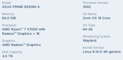
I am using Ubuntu as my operational system. Let's see if the OpenSSL is already installed. Usually, it is.

openssl version
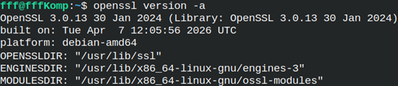	We can add option "-a" to get more information about OpenSSL. If your system doesn't have OpenSSL, you can easily install it with this line: sudo apt install openssl

OpenSSL Commands

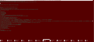
This is how we can list all of the OpenSSL commands.   openssl list -commands   This will show us all of the Standard, Digest and Cipher commands. It is also possible to limit this output to only those commands that interest us. openssl list -standard-commands openssl list -digest-commands openssl list -cipher-commands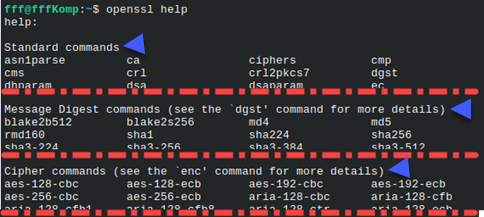

For specific command we can get help like this:   openssl dgst -help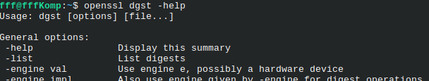

OpenSSL Man Pages

We can get Man pages for OpenSSL with this command. man openssl   For specific command we can see Man pages like this:   man openssl-dgst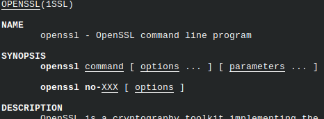

OpenSSL Hashing

I will first create one file, and I will place it on the Desktop.   seq 100 > /home/fff/Desktop/sequence1.txt   This file will contain numbers 1-100, although the content is not important.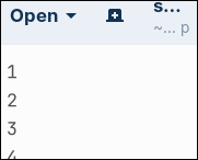

I will also create another version of this file that will have the number "9999" in the first line. I will name it "sequence2.txt".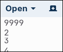

For hash creation, we will use "dgst" command. We can see on the image the hash that was created. We can run this command several times and each time we will get the same result. The hashing algorithm is deterministic.

cd /home/fff/Desktop openssl dgst -sha256 sequence1.txt
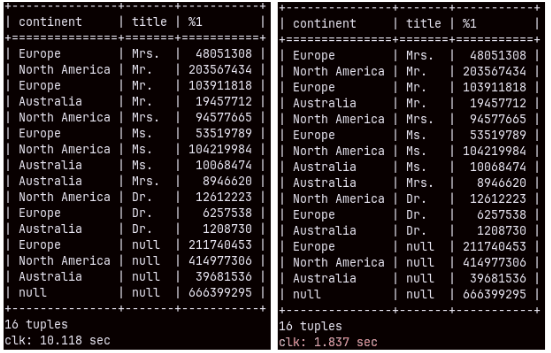
Currently we have files "sequence1.txt" and "sequence2.txt". They are almost the same. But their hashes will not be similar, they will be totally different. openssl dgst -sha256 sequence2.txt

All of the hashes will be of the same size, 64 hexadecimal characters. echo -n "Hello, World!" | openssl sha256

Hash Algorithms

We are using the command "dgst" to create a hash. We can also provide the hash algorithm. There are many algorithms, we used "sha256" algorithm.   We can get the list of hash algorithms with this command: openssl list -cipher-algorithms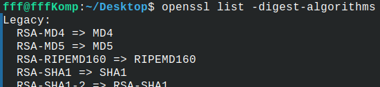

OpenSSL Encryption

This command will encrypt the file "sequence1.txt" by using "-aes-256-cbc" algorithm. We will be asked to enter our password twice. openssl enc -aes-256-cbc -in sequence1.txt -out sequence1.enc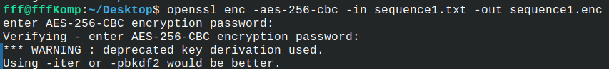

Notice that we are getting a warning to use "-iter" or "-pbkdf2". To encrypt data, AES algorithm must use 256-bit key, so the first step is to transform our password into this key, using hash algorithm. Transformation of the password into key is much more randomized if we use "-pbkdf2" option. We should always use it.

Salt

The hacker can create a collection of the most often used passwords. He can then use those passwords to brut force encrypted files. Because passwords are usually short, checking each password will only take a fraction of time. Our goal is to make this process more expensive.

Solution is to make passwords longer and more random. This can be done with a "salt". Salt is a random string that is concatenated to a password. Instead of the password being "pass123", now it will become "pass123KX8G#A". AES-256 key will be calculated by hashing this salted password.

Beside that, usage of "-pbkdf2" means that creation of AES-256 key takes more computational power. Thanks to salt and "pbkdf2", a hacker will need a few seconds to check each password. That will make impossible for him to brut force the password.

But who will provide the salt during the file decryption? The answer is that salt string "KX8G#A" will be saved together with an encrypted file. The "salt" itself is not encrypted. Anyone, who has encrypted file, can read the salt. When the user tries to decrypt the file, his password will be combined with a salt to generate salted password, that will be used for decryption.

Now, that we now about "-pbkdf2" and "-salt" we should add them to our command.

openssl enc -aes-256-cbc -pbkdf2 -salt -in sequence1.txt -out sequence1.enc     # the old file will be overwritten

Encrypted File

binary file

The result of the "enc" command will be a binary file. We can choose to generate "base64" encrypted file, if we use "-a" option. openssl enc -aes-256-cbc -pbkdf2 -salt -a -in sequence1.txt -out sequence1base64.enc Now, our file is textual file, we can copy-paste it anywhere =>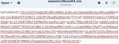

OpenSSL Decryption

For decryption we have to use "-d" option.                                                                                                                      openssl enc -d -aes-256-cbc -pbkdf2 -in sequence1.enc -out sequence1decr.txt	Because the key was created with "-pbkdf2" option, we must use it during the decryption.
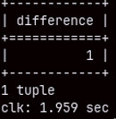
This command will confirm that there is no difference between the original and decrypted file. diff sequence1.txt sequence1decr.txt

Above, we decrypted binary file. For decrypting "base64" file we have to use "-a" option. openssl enc -d -aes-256-cbc -pbkdf2 -salt -a -in sequence1base64.enc -out sequence1base64.txt

Encryption Algorithms

This is how we can find the list of all of the encryption algorithms.   openssl list -cipher-algorithms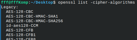

Symmetric vs Asymmetric Keys

When we used "enc" OpenSSL command, we only provided privacy. It is the same as if the users exchanged their files inside of the encrypted ZIP file. This kind of encryption is based on the symmetric keys, because there is a password that must be known by both of the parties.

For authentication, we must use asymmetric keys. In that case, there are two keys. One is the private key; the other is the public key. The private key is something that we hide and don't share with others. A person can use the private key to identify themselves.

To understand how private/public keys are related and generated, we'll look at the mathematics of the RSA algorithm for creating asymmetric keys. This isn't something we have to know, but it's really interesting to know.

RSA Algorithm

We will start by choosing two random prime numbers. I will choose 3 and 11. We will label them with P = 3 and Q = 11.

From P and Q we will calculate their product and their "Totient". "Totient" is a special mathematical property.	P	Q	N ( Product )	T ( Totient )
	3	11	P * Q = 3 * 11 = 33	( P – 1 ) ( Q – 1 ) = 2 * 10 = 20

Public Exponent "E"

P and Q will help us find E (the public exponent) and D (the private exponent). First, we will choose a public exponent. The public exponent must satisfy conditions below. The number 7 satisfies all of these conditions, so that will be our public exponent.

1) The public exponent E must be a prime number. 7 is a prime number.
2) It must be less than Totient ( 7 < 20 ).
3) Totient cannot be divided by the public exponent ( 20 / 7 = 2,857 ).

Private Exponent "D"

For private exponent "D" there is only one condition. This equation must be satisfied: "MOD( D * E, T ) = 1". There are many values for D that will satisfy this condition.	D = 3	MOD( 3 * 7, 20 ) = 1
	D = 23	MOD( 23 * 7, 20 )  = 1
	D = 43	MOD( 43 * 7, 20 ) = 1
	D = 63	MOD( 63 * 7, 20 ) = 1

Each time we increase the number D by +20, we get a candidate. I will use the smallest number D = 3.

RSA Encryption

I will encrypt number "16".

MOD( 16 ^ D, N ) = MOD( 16 ^ 3, 33 ) = 25

The number "16" encrypted is "25".

RSA Decryption

I will decrypt number "25".

MOD( 25 ^ E, N ) = MOD( 25 ^ 7, 33 ) = 16

The number "25" decrypted is "16".

For encryption, we need to know the private key. For decryption, we only need to know the public key. This property will help us use asymmetric keys for authentication.

Some Consideration for RSA Math

Modulus

When doing encryption and decryption we use Modulus function. We write Modulus function like this MOD(). This is the syntax that we use in spreadsheet programs. In mathematics we use different syntax:

MOD( 16 ^ D, N ) = 16 ^ D MOD N	This is the reason why in RSA terminology "Modulus" is a name for the number N. When we say "Modulus", we mean the number N.
MOD( 25 ^ E, N ) = 25 ^ E MOD N

Private and Public Key

For encryption we need private exponent D and Modulus N. Together they make a private key ( D, N ).

Similar to that, for decryption we need public exponent E and Modulus N. Together they are a public key ( E, N ).

Public Key is Derived from Private Key

This is something we hear often in lessons about cryptography. This is not true for RSA keys. For RSA keys, both keys are calculated based on the secret values for P and Q.

Every Asymmetric Key is Using One Way-Function

But where is the one-way function in the RSA algorithm? Let's say that the hacker knows the public key ( E, N ), and he wants to find the private key ( D, N ). Public key is not something that is a secret, only private key is secret.

Private key depends on Totient T. MOD( D * E, T ) = 1

Totient T depends on P and Q. ( P – 1 ) ( Q – 1 )

P and Q are factors of Modulus. P * Q = N

In the encryption example above we already saw that it hard to find P and Q, even with the help of a computer.

Modulus is calculated by the one-way function. It is easy to calculate N = f( P, Q ), but it is hard to calculate ( P, Q ) = f^-1( N ).

RSA Keys are Commutative

We can do encryption with private exponent D = 3, and we can do decryption with public exponent E = 7. It is also possible for them to reverse their roles. We can encrypt with 7, and decrypt with 3. This is something that is unique for RSA asymmetric keys.