Sort Your Pivot Table by Using Slicer

Sometimes different users want pivot table sorted in different ways. If column has full names of people, it is possible to sort column either by using first names or by using last names. An additional requirement is the ability to change the sort order using a slicer.

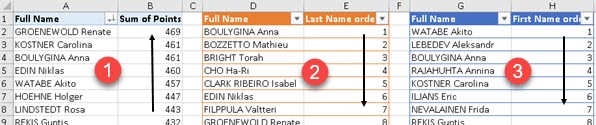
In the example bellow, we can see that our pivot table can be sorted by "Points" (1), but two other possible sorting orders are by "Last Name" (2) or by "First Name" (3). We will create solution only for this three specific sorting methods. Points will be sorted from highest to lowest, and first and last names will be sorted alphabetically.

Helper Tables

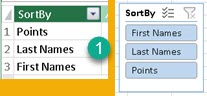First we have to create table in Power Pivot that will hold values for our slicer (1). We will call this table "SlicerValues".

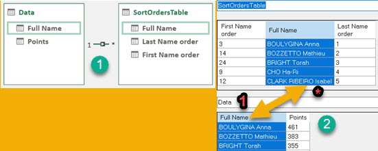
Second, we have to create table in Power Pivot, that will have columns with sort order for every row (1). We need two such columns, one for last names and one for first names. This table will have name "SortOrdersTable".

General Idea

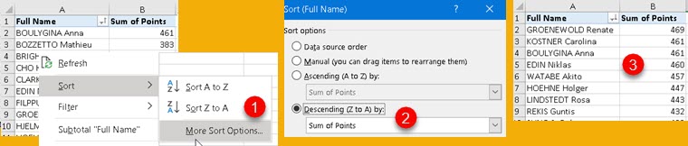
We know that it is possible to sort some column, in pivot table, by using some other column as sort order. First we have to right click on column which we want to sort, and then we go to Sort > More Sort Options (1). New dialog will open. In this dialog we will select "Descending (A to Z) by:" and then we will choose which column will define our sort order. In the image bellow, we decided that "Sum of Points" column (2) in DESC order is used for sorting. Now, "Full Name" column (3) is not sorted alphabetically, but according to "Sum of Points" column.

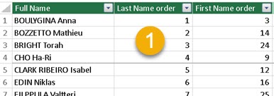
We can use mechanism, explained above, to control column "Full Name" sorting order. Idea is to create a measure, with a name "SortMeasure", that will be added to our pivot table (1). This measure values will change according to selection in the slicer (3,4,5). Our column "Full Name" will be set to sort by order defined by "SortMeasure" (2).

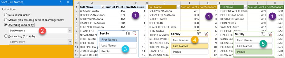
Now, when the user selects "First Names" (3), "Last Names" (4) or "Points" (5) in the slicer, column "SortMeasure" values will change (1) and that will sort our column "Full Name" (2). We can see in (3) that column "Full Name" is sorted by first name, in (4) by last name, and in (5) by points. At the end, column "SortMeasure" will be hidden from the user by hiding the whole spreadsheet column.

Creative process

First we have to make relation between "Full Name" columns in "SortOrdersTable" and "Data" table (1). "Data" table is the name of a table which is the base for our pivot (with "Full Name" and "Points" columns). Relation has to be "1:N" in direction "Data" to "SortOrdersTable" (2). This means that in relation dialog "Data" table has to be at the bottom. "Data" table can filter "SortOrdersTable".

Next step is to create our measure. This measure has to be reactive to slicer selection. ALLSELECTED function will return values selected in slicer as a column. With green part of code we will check whether specific individual values in slicer are part of that column. If they are, that means that those terms are selected and we will return TRUE(), otherwise we will return FALSE(). At the end, we will use SWITCH function to decide what values the measure should return. SWITCH function will return values for the first variable ( FirstNamesSelected, LastNamesSelected, PointSelected ) that returns TRUE(). For example, if FirstNamesSelected is FALSE(), and LastNamesSelected is TRUE(), values from "Last Name order" column will be returned. Those are the values that will be used to sort "Full Name" column.

SortMeasure:=
VAR FirstNamesSelected = IF( "First Names" IN ALLSELECTED( SlicerValues[SortBy] ); TRUE(); FALSE() )
VAR LastNamesSelected = IF( "Last Names" IN ALLSELECTED( SlicerValues[SortBy] ); TRUE(); FALSE() )
VAR PointsSelected = IF( "Points" IN ALLSELECTED( SlicerValues[SortBy] ); TRUE(); FALSE() )
VAR Result = SWITCH( TRUE(); FirstNamesSelected; SUM( SortOrdersTable[First Name order] ) 
                           ; LastNamesSelected; SUM( SortOrdersTable[Last Name order] )
                           ; PointsSelected; 10000 - SUM( Data[Points] ))
RETURN Result

All columns with possible result ( "First Name order", "Last Name order", "Points" ) are just wrapped in SUM function, but "Points" column has one more detail. In our measure we will transform all "Points" values into "10000 – Points". This is because, we want ascending sorting for "First Name order" and "Last Name order", but descending sorting for "Points". Because pivot table can only be in ascending or descending order at once, we need this transformation so that ascending ordering of our measure will always correctly sort our pivot table. Values of "Points" and "10000 – Points" are inversely correlated, and this solves our problem.

Descending sorting of "Points" is the same as ascending sorting of a transformation "10000 – Points".

Result

Bellow we can see our results and we can observe a few details. Columns "C" and "G" are hidden (1). This is how we will hide our "SortMeasure" column from the user. In green pivot table (2) we can see that while "SortMeasure" column is in ascending order, important column "Sum of Points" is actually in descending order, as per requirement.

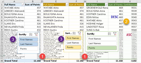
In blue and orange pivot tables, there are two values selected in each slicer (3). It is not possible to force single selection in slicer in Excel without resorting to VBA. To solve this problem, we made our measure so that the first selected value is the one determining sorting order. That is why both blue and orange pivot tables are sorted by "First Names", that is the first value selected in their slicers.

Sample table can be downloaded from here: