SPSS / By Bizkapish
/ November 6, 2022 November 6, 2022
We saw in one of earlier posts what are descriptive statistics. Let's see how to calculate those statistics in SPSS.
Descriptive Statistics Dialogs
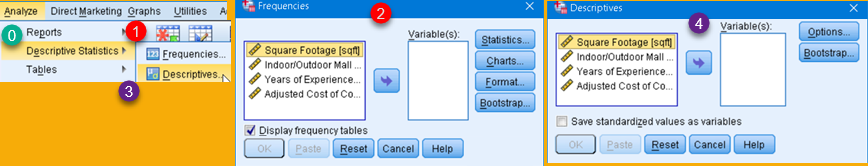
SPSS has two similar dialogs for creation of descriptive statistics. Both dialogs can be called from menu Analyze > Descriptive Statistics (0). There we can choose option Frequencies (1) to get dialog (2), or we can choose Descriptives (3) to get dialog (4). Dialogs (2,4) are similar. Dialog Frequencies gives us more options than dialog Descriptives.
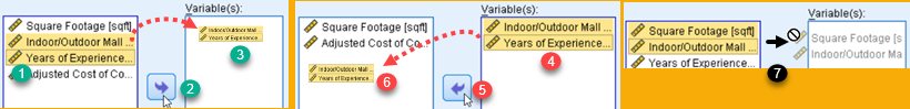
First step is to select columns for which we will calculate descriptive statistics. By using mouse, and keys Ctrl or Shift, we should select some of the columns from the first pane (1). Then we will click on button (2) so that columns are moved to second pane (3). These are the columns for which we will get our descriptive statistics.
If we had made a mistake, it is possible to move columns from the right pane to the left pane, by using the same process (4,5,6). It is also possible to move selected columns to opposite pane by dragging and dropping with mouse (7).
Analyze > Descriptive Statistics > Frequencies
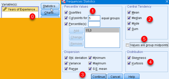
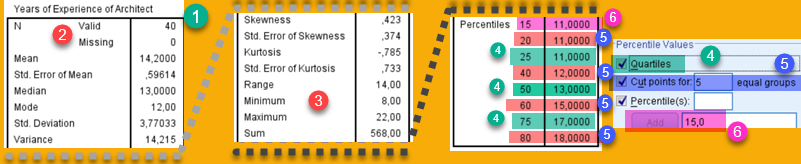
In Frequencies dialog, we should click on "Statistics" button (0). This will open new dialog where we can choose what descriptive statistics should be calculated. We can choose Percentiles (1), Central Tendency statistics (2), Measures of Variability (3), and Distribution (4).
Option (5) "Values are group midpoints" is used when our source data is grouped and each group is presented by one value. For example, all people in their thirties are coded as value 35. In that case this option "Values are group midpoints" will estimate Median and Percentiles for original, ungrouped data.
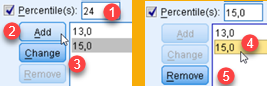
Custom percentiles are added by typing them into textbox (1) and then we click on "Add" (2). This will add that percentile ("24") to the pane bellow. If we click on "Change" (3) then the new value ("24") will replace currently selected old value ("15"). If one of the values (4) is selected then we can remove that value with button "Remove" (5).
Now we can click Continue and OK to close all dialogs and SPSS will calculate our results. All the results will be presented in one tall table (1). On the top we can see valid and missing values (2). Missing values are nulls. Bellow are all the others statistics that we are already familiar with (3).
At the bottom of the table, we have percentiles. All the percentiles are presented together (4,5,6). I've color-coded the percentiles here to help us understand the "Percentile Values" options. If we check option "Quartiles" (4), we will get percentiles 25, 50, 75. Option (5) allow us to divide 100% to several groups of equal size in %. If we want to get 5 groups, then 100% will be divided by using 4 cut points. Those cut points are 20, 40, 60 and 80 . At last, we will see all custom percentiles we have entered (6).
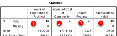
For several selected variables result would be presented as new columns in the result table. Order of columns will be the same as order of selected variables.
Analyze > Descriptive Statistics > Descriptives
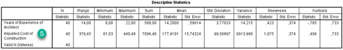
If we use Descriptives dialog, process is similar. First, we select our columns (3) and then we click on button (1). This will open dialog (2) where we can select what descriptive statistics should be calculated.
Final result will be presented in one table where each variable will have its results presented in one row. Order of rows can be controlled by options (4). Default is to use "Variable list" as order of columns (5).
SPSS / By Bizkapish
/ August 14, 2022 November 6, 2022
Descriptive statistics is a branch of statistics that is describing the characteristics of a sample or population. Descriptive statistics is based on brief informational coefficients that summarize a given data set. In descriptive statistics we are mostly interested in next characteristics:
Frequency Distribution or Dispersion, refers to the frequency of each value.
Measures of Central Tendency, they represent mean values.
Measures of Variability, they show how spread out the values are.
Frequency Distribution
Frequency distribution shows how many observations belong to different outcomes in a data set. Each outcome can be described by group name for nominal data or ordinal data, interval for ordinal data or range for quantitative data. Each outcome is mutually exclusive class. We just count how many statistical units belong to each class.
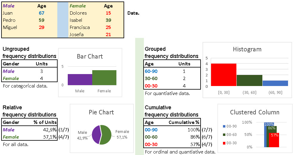
Frequency distribution is usually presented in a table or a chart. There are four kinds of dispersion tables. For each kind of table there is a convenient chart presentation:
– Ungrouped frequency distributions tables show number of units per category. Their counterpart is Bar Chart. – Grouped frequency distributions tables present number of units per range. Their companion is Histogram. – Relative frequency distributions tables show relative structure. Their supplement is Pie Chart. – Cumulative frequency distributions tables are presenting accumulation levels. Their double is Clustered Column chart.
Measures of Central Tendency
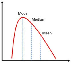
Measures of central tendency represent data set as a value that is in the center of all other values. This central value represents the value that is the most similar to all other values and is the best suited to describe all other values through one number. There are three measures of central tendency, Average, Median and Mode. In normal distribution these three values would be the same. If we don't have symmetry, then Median would be closer to extreme values then the Average, and Mode be at the top of distribution.
Average
Average is calculated by summing all the values, and then dividing the result with number of values ( x̄ = Σ xi / n ).
Median
The median is calculated by sorting a set of data and then picking the value that is in the center of that array. Let's say that all values in array are indexed from 1 to n [ x(1), x(2)…x(n-1), x(n)].
If number of values in array is odd, median is decided by index (n+1)/2. Median is then decided like x̃ = x(n+1)/2, like in array [ 9(1), 8(2), 7(3), 3(7+1)/2, 1(5), -5(6), -12(7)]. There are an equal number of values before and after median in our array, 3 values before the median and three values after the median.
If number of values is even, formula is x̃ = (x(n/2)+x(n/2)+1)/2, like in [ -3(1), 1(2), 0(3), 2(8/2), 3(8/2)+1, 4(6), 6(7), 9(8)], so we calculate an average of two middle numbers (2+3)/2 = 2.5. Again, there are an equal number of values in our array before and after the two centralvalues. As we can see, it is not important whether numbers are arranged in ascending or descending order.
Mode
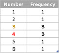
The mode is the most frequent value in a sample or population. One data set can have multiple modes. In sample ( 1, 3, 2, 3, 3, 5, 4, 4, 8, 4 ) we have two modes. Both the numbers 3 and 4 appear three times. If we create Ungrouped Frequency Distribution table, we can easily notice our modes.
Measures of Variability
Measures of Variability shows how spread out the statistical units are. Those measures can give us a sense of how different the individual values are from each other and from their mean. Measures of Variability are Range, Percentile, Quartile Deviation, Mean Absolute Deviation, Standard Deviation, Variance, Coefficient of Variation, Skewness and Kurtosis.
Range
Range is a difference between maximal and minimal value. If we have a sample 2, 3, 7, 8, 11, 13, where maximal and minimal values are 13 and 2, then the range is: range = xmax– xmin= 13 – 2 = 11.
Percentile
Let's say that we have sample with 100 values ordered in ascending order ( x(1), x(2)…x(99), x(100) ). If some number Z is bigger than M% values from that sample, than we can say that Z is "M percentile". For example, Z could be larger than 32% of values ( x(1), x(2)… x(32), x(33), x(99), x(100) ). In this case x(33)is "32 percentile".
For this sample [ -12(1), -5(2), 1(3), 3(4), 7(5), 8(6), 9(7)], number 7 is larger than 4 values, so seven is "57 percentile". This is because 4 of 7 numbers are smaller than 7, and 4/7 = 0,57 = 57%. Percentile show us how big part of sample is smaller than some value.
Be aware that there are several algorithms how to calculate percentiles, but they all follow similar logic.
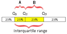
Percentiles "25 percentile", "50 percentile", "75 percentile" are the most used percentiles and they have special names. They are respectively called "first quartile", "second quartile" and "third quartile", and they are labeled with Q1, Q2, Q3. Quartile Q2 is the same as median.
Quartiles, together with maximal and minimal values divide our data set in 4 quarters. xmin [25% of values] Q1[25% of values] Q2[25% of values] Q3[25% of values] xmax
Quartile Deviation
The difference of third and first quartile is called "interquartile range": QR = Q3 – Q1. When we divide interquartile range with two, we get quartile deviation. Quartile deviation is an average distance of Q3 and Q1 fromthe Median.
Average of ranges A and B is quartile deviation, calculated as: QD = (Q3 – Q1 ) / 2.
Mean Absolute Deviation
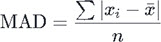
Mean absolute deviation (MAD) is an average absolute distance between each data value and the sample mean. Some distances are negative and some are positive. Their sum is always zero. This is a direct consequence of how we calculate the sample mean.
x̄ = Σ xi / n n * x̄ = Σ xi n * x̄ – ( n * x̄ ) = Σ xi – Σ x̄ 0 = Σ ( xi – x̄ )
We can see, on the left, that formula, used for calculation of a mean, can be transformed to show that sum of all distances between values and the mean is equal to zero. This is why, for calculating mean absolute deviation (MAD) we are using absolute values.
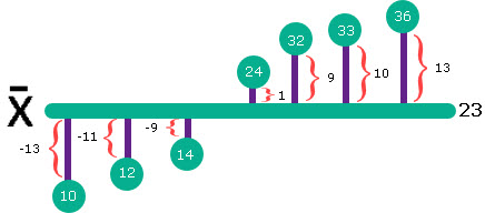
If our sample is [ 10, 12, 14, 24, 32, 33, 36 ], mean value is 23. Sum of all distances is ( -13 – 11 – 9 + 1 + 9 + 10 +13 ) = 0. Instead of original deviations we are now going to use their absolute values. So, sum of all absolute deviations is ( 13 + 11 + 9 + 1 + 9 + 10 + 13 ) = 66. This means that MAD = 66 / 7 = 9,43.
Standard Deviation and Variance
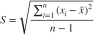
The standard deviation is similar to the mean absolute deviation. SD also calculates the average of the distance between the point values and the sample mean, but uses a different calculation. To eliminate negative distances, SD uses the square of each distance. To compensate for this increase in deviation, the calculation will ultimately take the square root of the average squared distance. This is the formula used for calculating standard deviation of the sample:
Variance is just standard variation without root =>
Standard deviation is always same or bigger than mean absolute deviation. If we add some extreme values to our sample, then standard deviation will rise much more than mean absolute deviation.
Coefficient of Variation
Coefficient of variation is relative standard deviation. It is a ratio between standard deviation and the mean. The formula is CV = s / x̄. This is basically standard deviation measured in units of the mean. Because it is relative measure, it can be expressed in percentages.
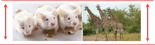
Let's imagine that the standard deviation of a giraffe's height is equal to 200 cm. Standard deviation of a mouse's height could be 5 cm. Does that mean that variability of giraffe's height is much bigger than variability of mouse's height? Of course it is not. We have to take into account that giraffes are much bigger animals than mice. That is why we use coefficient of variation.
If we scale the images of mice and giraffes to the same height, we can see that the relative standard deviation of their heights is not as different as the ordinary standard deviation would indicate.
Kurtosis and Skewness
Kurtosis and Skewness are used to describe how much our distribution fits into normal distribution. If Kurtosis and Skewness are zero, or close to zero, then we have normal distribution.
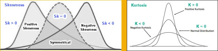
Skewness is a measure of the asymmetry of a distribution. Sometimes, the normal distribution tends to tilt more on one side. If skewness is positive then distribution is tilted to right side, and if it is negative it is tilted to left side.
If skewness is absolutely higher than 1, then we have high asymmetry. If it isbetween -0,5 and 0,5, then we have fairly symmetrical distribution. All other values mean that it is moderately skewed.
To the right we can see how to calculate Skewness statistics.
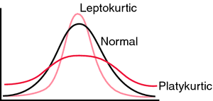
The Kurtosis computes the flatness of our curve. Distribution is flat when data is equally distributed. If data is grouped around one value, then our distribution has a peak. Such humped distributions mean that kurtosis statistics is positive. That is Leptokurtic distribution. Negative values of kurtosis would mean that distribution is Platykurtic. The distribution is then more flat. Critical values for kurtosis statistics are the same as for skewness.
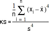
To the right we can see how to calculate Kurtosis statistics.
An observational unit is the person or thing on which measurements are taken. Observational units have to be distinct and identifiable. Observational unit can also be called case, element, experimental unit or statistical unit. Examples of observational units are students, cars, houses, trees etc. An observation is a measured characteristic on an observational unit.
All observational units that have one or more characteristics in common, are called population. For example, if we observe people, all the people in one country can make population. They are all sharing the same characteristic that they are residents of the same country. One observational unit can belong to several populations at the same time, depending on the characteristics used to define those populations.
Sample is a subset of population units.
Population is a set of elements that are object of our research. Sampling is observing only subset of the whole population. Sample is always smaller then population, so it is really important for sample to be representative, it should have the same characteristics as the population.
Parameter is a function, that uses observations of all units in population, to calculate one real number. That real number represents value of some characteristic of the whole population. For example, if we have measured height of all the people in one population, we can use function μ = ( Σ Xi ) / N, to calculate average height. For specific given population, parameter is a constant that is result of parameter function.
Statistic is the same as Parameter, but it is calculated on a sample. Example would be function x̄ = ( Σ xi ) / N. When statistics is used as an estimate for a parameter, it is referred as an estimator.
Method (random, stratified, cluster…) used to select the observation units from a population into sample is known as sampling procedure. When we decide what sampling procedure and what statistics to use in our research, those two decision together created our sampling design.
For some sampling procedures we need to create list of all observation units that comprise that population. Such list is called frame or sampling frame.
Benefits and disadvantages of sampling
Benefits of sampling are: – Research can be conducted faster and with smaller cost. Organizational problems could be avoided. – Sometimes it is not possible to observe whole population. Some observational units are not accessible, or there is not enough highly trained personnel of specialized equipment for data collection. Sometimes we don't have enough time to observe full population. – When sample is smaller, personnel can be better trained to produce more accurate results. – Personnel could dedicate more time to one observational unit. They can measure many characteristics of a unit, so data can be collected for several science projects at the same time.
Collection of information on every unit in the population for the characteristics of interest is known as complete enumeration or census. Census would give us correct results. If we use sampling we can make mistakes like: – Our results could be biased. This is consequence of the wrong sampling procedure. – If phenomena under study is complex, it is really hard to select representative sample. Some inaccuracy will occur. – Sometimes it is impossible to properly collect the data from observation units. Some respondents will be not reachable, they will refuse to respond or they are not capable of responding. This would force us to find replacements for some observation units. – Sampling frame could be incorrect and incomplete. This is often the case with voters list.
Steps in sampling
Define the population. The definition should allow researcher to immediately decide whether some unit belongs to population or not.
Make a sampling frame.
Define the observation unit. All observation units together should create population. Observation units should not be overlapping, they should be exclusive.
Choose a sampling procedure.
Determine the size of a sample based on sampling procedure, cost, and precision requirements.
Create a sampling plan. Sampling plan is detailed plan of which measurements will be taken, on what units, at what time, in what way, and by whom.
Select the sample.
Types of sampling procedures
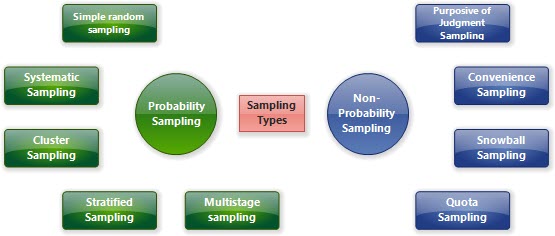
There are two groups of sampling methods. Those are Probability Sampling and Non-Probability Sampling. – Probability Sampling involves random selection where every element of the population has an equal chance of being selected. If our sample is big and randomly selected that would guarantees us that our sample is representative. Unfortunately, this is not so easy to accomplish. – Non-Probability Sampling involves non-random selection where the chances of selection are not equal. It is also possible that some units have zero chance to be included in the sample. We use this method when it is not possible to use Probability Sampling or when we want to make sampling more convenient or cost effective. Such sampling methods are often used in preliminary stages of research.
Probability Sampling procedures
Simple Random Sampling
Simple random sampling requires that a list of all observation units be made. After this, we select some of observation units from that sampling frame by using either lottery technique or random numbers generator.
Sampling frame should be enumerated so that we can use five random numbers to select five Countries from our frame above.
Advantages of Simple Random Sample are: – It is simple to implement, no need for some special skills. – Because of its randomness, sample will be highly representative.
Disadvantages of Simple Random Sample are: – It is not suitable for large populations because it requires a lot of time and money for data collection. – This method offers no control to researcher so unrepresentative samples could be selected by chance. This method is best for homogenous populations where there is smaller risk to create biased sample. This could be solved only by bigger samples. – It could be difficult to create sampling frame for some population. – This method doesn't take in account existing knowledge that researcher has about population.
Systematic Sample
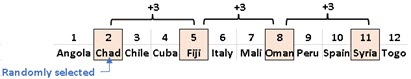
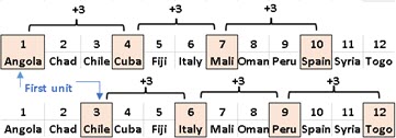
Systematic sample asks for population to be enumerated. If population has 12 units, and the size of sample is 4, we want to select one observation unit in every three (=12/4) consecutive units. The first element should be randomly selected in the first three observation units. We will select element 2 in our image below. After this, we will select every third unit. At the end, units 2,5,8 and 11 will create our sample.
In Systematic Sample first unit is randomly selected and others are selected in regular intervals.
Two other possible samples could start on first and on third element.
Advantages of Systematic Sample are: – Systematic Sample is simple and linear. – Chance of randomly selecting units that are close in population is eliminated. – It is harder to manipulate sample in order to get favored result. Systematic Sample rigidly decide which units will become part of a sample and which will not. This is only true if we have some natural order of units. If researcher can manipulate how units are ordered, then it could be actually easier for him/her to manipulate results.
Disadvantages of Simple Random Sample are: – We have to know in advanced, how big is our population, or at least we have to estimate its size. – If there is a pattern in units order, Systematic Sample will be biased. For example, if we choose every 11-th player in some football cup, we could actually select only goalkeepers. No regular player would be selected. We should avoid populations with periodicity.
Cluster Sampling
Cluster Sampling can be used when whole population could be divided into groups where each group has the same characteristics as the whole population. Such groups are called clusters. We can randomly select several clusters and they will comprise our sample.
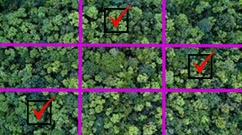
Imagine that we want to investigate trees in some forest. We don't have to encompass all the trees. We can divide forest into parcels. We can then select several parcels and only trees in those parcels will be object of our research.
Advantages of Cluster Sampling are: – Observation units could be spatially closer to each other. In our example, all the trees on one parcel are in proximity of each other. This could significantly reduce cost of data collection. – Because observation units are close to each other it is easier to create and collect bigger samples. – If clusters really represent population, estimates made with cluster sampling will have lower variance.
Disadvantages of Cluster Sampling are: – We have to be careful not to include clusters that are different then general population. – Units shouldn't belong to several clusters. In our example, one tree can be on the border between parcels. We could measure it twice. – It is statistical requirement that all clusters should be of similar size.
Stratified Sampling
Stratified Sampling involves dividing the population into subpopulations that may differ in some important trait. Such subpopulations should not overlap and together they should comprise the whole population. One such subpopulations is called stratum. Plural of the word stratum is strata. After this, we should take simple random of systematic sample from each stratum. Number of units taken from each stratum should be proportional to the size of the stratum.
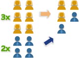
Here, we divided our population based on gender. In our population ratio between men and women is 3:2. The same ratio should stay inside of our sample. If our population has 6 women and 4 men, then our sample should have 3 women and 2 men, if the size of sample is 5 in total.
Advantages of Stratified Sampling are: – Every important part of population is included in sample. – It is possible to investigate differences between stratums. – Because units in each strata are similar, average value of some characteristic of those units will have smaller variance. This will have as consequence that variance of estimator for the whole population will have smaller variance too.
Disadvantages of Stratified Sampling are: – We need to make complete sampling frame. Each observation unit has to be classify in which stratum belongs. – Often it is hard to divide population in subpopulations that are internally homogenous but are heterogenous between them.
Multistage Sampling
Multistage Sampling is a method of obtaining a sample from a population by splitting a population into smaller and smaller groups and taking samples of individuals from the smallest resulting groups. Multistage Samplinginvolves stacking multiple sampling methods one after the other. Stratified Sampling is a special case of Multistage Sampling because it has two stages. One other possible method could be to divide population into clusters and then to take systematic sample from each cluster.
Non-Probability Sampling procedures
Purposive of Judgment Sampling
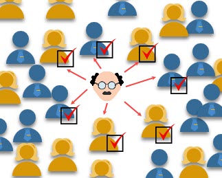
Judgmental sampling is when the researcher have right to discretely selects the units of the sample, by using their knowledge. It is used when researcher wants to gain detailed knowledge about some phenomenon. It is also used when population is very specific and hard to identify.
You want to interview winners of lottery about how they are spending and investing their money. Well, there are not so many winners of lottery and many of them will refuse to speak with researcher or their identity is a secret. Examiner will not find many people to talk with. In that case, every winner willing to share their experience will become part of purposive sample.
Another example would be when researcher interview only people who gave the most representative answers in some previous research or he/she wants to interview only people which have enough knowledge to predict some future event.
Advantages of Purposive Sampling are: – It can be used for small and hidden populations. – Examiner can use all of his knowledge to create heterogenous and representative sample. – This sampling method can combine several qualitative research designs and can be conducted in multiple phases.
Disadvantages of Purposive Sampling are: – There is huge bias because sample is not selected by chance. Also, when we use purposive sampling, our sample is usually small. – There is no way to properly calculate optimal size of sample or to estimate accuracy of the research results. – Examiner can easily manipulate the sample to get artificial results.
Convenience sampling
In this sampling procedure, units are selected based on their availability and willingness to take part. Studies that rely on volunteers or studies that only observe people on convenient places like busy streets, malls or airports are examples of Convenience Sampling. This technique is known as one of the easiest and cheapest.
Advantages of Convenience Sampling are: – We can collect answers from dissatisfy buyers or employees. People are hesitant to express their dissatisfaction openly but they are more willing to do it during some research. – This method is good for first stages of research because we don't have to worry about quality of our sample, all participants are willing to give us answers, we can collect some demographic data about them, we can get immediate feedback. – It is cheap and fast.
Disadvantages of Convenience Sampling are: – Potential bias. We are only covering people and things near to us, all others will be neglected. Results from convenience sampling can not be generalized. – People who are in a hurry will often give us incomplete or false answers to shorten the interaction with us. This can cause the examiner to start avoiding people who are nervous or in a hurry and thus further reduce the representativeness of the sample.
Snowball Sampling
For Snowball Sampling we have to start with only few participants. Those people are asked to nominate further people known to them so that the sample increases in size like a rolling snowball. This technique is needed when participants don't want to talk about their situation because they feel vulnerable or in danger. Such populations are homeless, illegal immigrants, people with rare diseases.
Advantages of Snowball Sampling are: – It can be used when sampling frame is unknown, when respondents don't want to disclose their status or to identify themselves. – Sampling process is faster and more economical because existing contacts are used to reach to other people.
Disadvantages of Snowball Sampling are: – Because they are connected, all participants have some common traits. This can exclude all other members of our population who don't share those traits. This means that there is huge bias in our research because population is not correctly presented. – People from vulnerable groups can show resistance and doubt. Researcher has to be careful to earn their trust. – Examiner can not use his previous knowledge to make sample better. He can not control the sampling process.
Quota sampling
Quota Sampling is similar to stratified sampling. Here, we also try to split population in exclusive homogeneous groups. This way we reduce variance inside such groups. After this, we apply some non-probability sampling method to select units inside our strata.
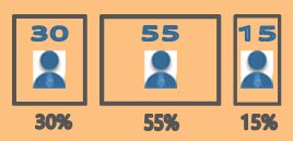
We don't know how big is our population, nor do we know how big are strata. Instead of that we are trying to guess what percentage of general population makes each of strata, based on some older research or on our expertise. We also have to decide how big our sample should be. Because samples from each stratum should be proportional to stratum size, we have enough information to decide how many units to pick from each stratum. If our strata are in proportion of 30% : 55% : 15%, and we want sample of 100 units then we have to choose 30, 55, 15 units from each stratum respectively.
Advantages of Quota Sampling are: – Quota Sampling is simpler and less demanding on resources, similar to other non-probability sampling methods. – Scientist can increase precision of research by proper segmentation of population by using his knowledge. – We don't need to have sampling frame.
Disadvantages of Quota Sampling are: – Like other non-probability methods, Quota Sampling introduce bias but that could be mitigate by proper partition of population.
SPSS / By Bizkapish
/ January 30, 2022 January 30, 2022
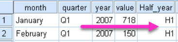
Recoding is process of transforming variable values by using some rule. Simple example would be that we want to replace quarter of the year values (Q1,Q2,Q3,Q4) with half of the year values (H1,H2).
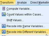
As a result we can create new variable (as on the image above) or we can overwrite existing variable. This depends on whether we open dialog Transform > "Recode into Same Variables" or "Recode into Different Variables".
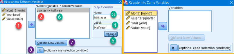
Both options will open similar dialog. The difference is that "Recode into Same Variables" will not have textboxes (3,4) and button (5) because there will be no new variable. This is the only difference so we will explain only "Recode into Different Variables" case.
First, we choose column to recode (1) and we add it to pane (2). Next, we give name and label to the new column (3,4). After that, we click on the "Change" button (5) and name of the new column will be added to pane (6). Now we have to define how new column will be created. For that we use dialogs "Old and new Values" (7) and "If…" (8).
System Missing and User Missing Values
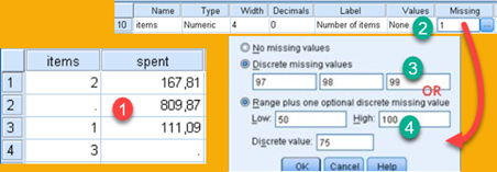
This terms are used in dialog "Old and New Values". If we have some values missing in our data source, SPSS will present such values with a dot (1). Those are called System Missing Values.
Other possibility is for user to declare some values as invalid or impossible. This is done in "Variable view" (2). In new dialog user will enter three discrete values (3), or combination of one range and one discrete value (4). Invalid values will not be specially labeled in "Data view", but rows with such values will be excluded from any further analysis by the SPSS. This is explained in the blog post https://bizkapish.com/spss/spss-data-entry/.
Old and New Values
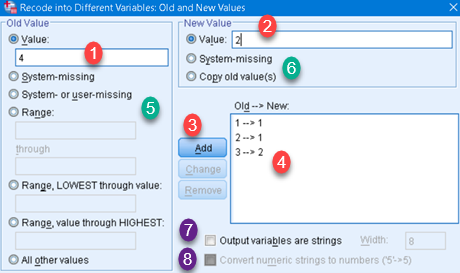
We want to transform quarter of year values (coded as 1,2,3,4) to half of year values (coded as 1,2). We enter code of a quarter in (1), and code of a half of year in (2). Then we click on button "Add" (3) and new transformation will appear in pane (4). We have to do this for each combination of quarter and half of year. We also have option to change the type of a result value. We can change it from number to string (7), or from string to number (8), if possible.
"Old and new values" dialog has left (5) and right (6) side. On the left side we can choose to transform specific value, missing values, range of vales, or all other values. On the right side we can choose to transform those values into specific value, missing value or just to copy old values. So, anything selected on the left side can be transformed to anything selected on the right side.
Conditional selection
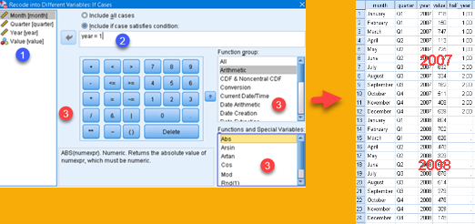
We can make transformations conditional. For that we use "If…" dialog. In this dialog we use columns (1) to create expression (2). Transformation will occur only in those rows where this expression returns true. We can type expression manually, but we can also use any of the controls (3) to add building blocks in our expression. This is better explained in the post https://bizkapish.com/spss/how-to-create-new-variables-in-spss/.
In image above we typed expression "year = 1". This means that only quarters in the year 2007. will be transformed to half years. Rows for 2008. will be missing (presented by dot). If we want to fill cells for 2008. we have to create new transformation, but this transformation has to use the same name of new variable .
Let's say that we want to perform three conditional transformations. Each next transformation will overwrite cells where its condition is fullfiled. If there is overlap in some rows for two transformations, the last transformation will prevail. See the image. In the last step we change our transformation to "9", just to make a difference.
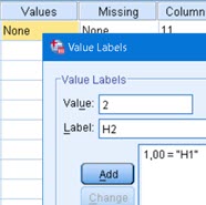
Value Labels
Last step is to associate new code values with their text labels. This is done in usual way, in "Variable view".
SPSS / By Bizkapish
/ December 4, 2021 December 4, 2021
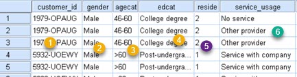
Our table has data about cable television users. We have ID of the customers (1), their gender (2), age group (3) and education level (4). Column "reside" (5) shows how many people live in the household. Column "service_usage" (6) shows what kind of cable service they use. We will see how to filter this data in different ways in SPSS program.
On the image on the right we can see that filtering dialog is opened by clicking on Data > Select Cases (1). This opens dialog where we can select columns to filter (2), we can choose how to filter (3), and we can decide what will happen with filtered data(4).
5 ways to filter data
All cases
"All cases" option means that there will be no filtering. This is the default.
If condition is satisfied
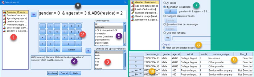
This option opens dialog where we can define formula that will filter data. We can click on column names (1), math and number symbols (2), and we can choose some of built-in functions (3). What we click, will appear in pane (6). We can also type by hand what we want in pane (6). Whole expression can be typed manually, but it is more easier to select elements of expression. Pane (5) will filter functions presented in the pane (3). This will help us to find function we want. When we select one of the functions in the pane (3), we can see its syntax and description in the pane (4).
Now that we created our filter (7), we will choose to "Filter out unselected cases" (8). This option will not hide or delete filtered data (9), but will only mark it as filtered (10). Although still visible, marked rows will not be included in SPSS calculations. This way we don't loose any data and we can after, apply some other filter on our table.
Random sample of cases
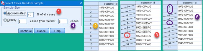
Button "Sample" opens dialog where we can use one of two possible random filters. First filter (1) will choose some percent of all the cases randomly. For this to show, I will use smaller table that has only 10 rows (2). If we choose to filter 10% of rows, only one row will be left (3). Other option (4) is to randomly select a limited number of rows from the specified number of first cases. We choose to select 3 rows from the first 5 rows, so only rows 1, 2 and 5 will be selected (5).
Base on time or case range
We can just choose one continuous range of cases. On image left, we can see (1) that we have chosen all cases between case 3 and 7 inclusively. All other cases will be crossed out (2).
Use filter variable
This option asks from us to select one of the columns (1). This column should have rows without data (2). All the rows where that columns doesn't have data will be filtered (3).
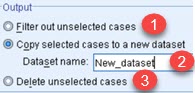
What will happen with filtered data?
Filtered data can be marked as filtered out and such rows will be excluded from further calculations (1). There are two more options. First is to create new Dataset(2). SPSS will open a new window. That window will show all the rows, but unselected rows will be crossed out. Other possibility is to delete cases that don't pass filter condition. Our Dataset will be then reduced by deleting not needed rows (3). You should be careful when deleting the rows because deleting can not be undone.