Power BI Desktop

Our Model

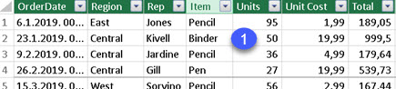
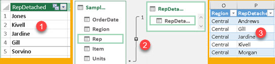
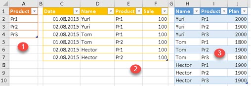
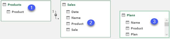
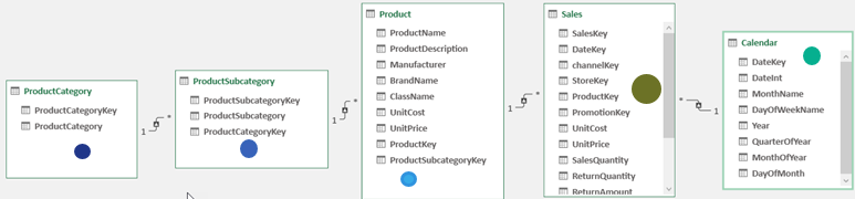
We will use this simple model to explain SUMMARIZECOLUMNS function. On the left side we have ProductCategory > ProductSubcategory > Product. On the right side we have "Calendar" table. "Sales", the fact table is in the middle.

Grouping Columns

In its simplest form, this function just groups values from several columns. If the columns do not belong to the same table, the result will be a cross join of their values.

EVALUATE SUMMARIZECOLUMNS(         ProductCategory[ProductCategory]    , Calendar[Year] ) ORDER BY ProductCategory[ProductCategory]               , Calendar[Year]

But if the columns are from the same table, then only distinct rows of those columns will be returned.

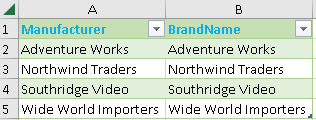
EVALUATE SUMMARIZECOLUMNS(      Product[Manufacturer]    , Product[BrandName] ) ORDER BY Product[Manufacturer]                , Product[BrandName]

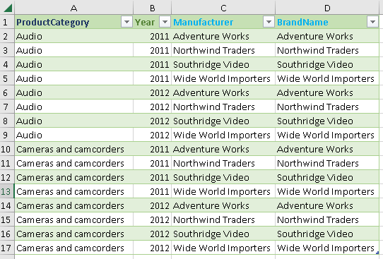
If the first table above has 24 rows, and the second has 4 rows, then the formula below will give us a table with 4 * 24 = 96 rows. The formula below combines all four columns.

EVALUATE SUMMARIZECOLUMNS( ProductCategory[ProductCategory], Calendar[Year]                                     , Product[Manufacturer]                    , Product[BrandName] ) ORDER BY                      ProductCategory[ProductCategory], Calendar[Year]                                     , Product[Manufacturer]                    , Product[BrandName]

Filter Table Argument

We don't need to combine all the values from the columns, we can apply filters on them. Any table mentioned after grouping columns will be considered as a filter.

this is filter table created with TREATAS function. This is why we only have two categories in our table.

EVALUATE SUMMARIZECOLUMNS(      ProductCategory[ProductCategory]    , Calendar[Year]    , Product[Manufacturer]    , Product[BrandName]    , TREATAS( { "Audio", "Cameras and camcorders" }         , ProductCategory[ProductCategory] ) ) ORDER BY ProductCategory[ProductCategory]               , Calendar[Year]               , Product[Manufacturer]               , Product[BrandName]

It is possible to use several filter tables. Each table will filter the columns that belong to it.

We now have two filter tables created with TREATAS function. One will apply a filter to the "ProductCategory" column, and the other  to the "Year" column.

EVALUATE SUMMARIZECOLUMNS(      ProductCategory[ProductCategory]    , Calendar[Year]    , Product[Manufacturer]    , Product[BrandName]    , TREATAS( { "Audio", "Cameras and camcorders" }         , ProductCategory[ProductCategory] )    , TREATAS( { 2011, 2012 }, Calendar[Year]   ) ) ORDER BY ProductCategory[ProductCategory]               , Calendar[Year]               , Product[Manufacturer]               , Product[BrandName]

The grouping column must be part of the filter table, for the filter to apply.

Aggregations

Now we can add some aggregations. Aggregations are defined by the the name of the new column, and then we add some expression that returns a scalar value.

The SUMMARIZECOLUMNS function was born for this. This is the fastest and easiest function to group columns from several tables and then add some aggregated values from a fact table. A lot of work can be done with just one function.

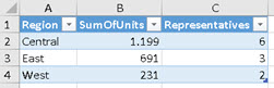
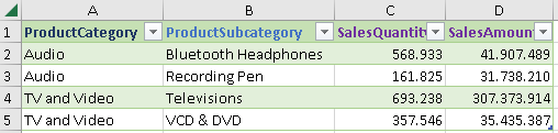
*In the source data, we only have Sale for this two product categories.

EVALUATE SUMMARIZECOLUMNS(      ProductCategory[ProductCategory]    , ProductSubCategory[ProductSubCategory]    , "SalesQuantity", SUM( Sales[SalesQuantity] )    , "SalesAmount", SUM( Sales[SalesAmount] )   ) ORDER BY ProductCategory[ProductCategory]                , ProductSubcategory[ProductSubcategory]

NONVISUAL

Filter Table argument can do two things. It can affect the number of rows, and it can also affect the measurements. Let's make one measure:
TotalSalesAmount:=SUM( Sales[SalesAmount] )

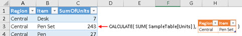
As you can see below, we just summed the two subcategories with the measure TotalSalesAmount ( 339.112.125 ). The measure is influenced by the filter table argument. We can notice that if we display all the data, then the total amount of sales would be 416.455.001.

EVALUATE SUMMARIZECOLUMNS(      ProductSubcategory[ProductSubcategory]    , TREATAS( { "Recording Pen", "Televisions" }         , ProductSubcategory[ProductSubcategory] )    , "SalesQuantity", [TotalSalesAmount]    , "SalesAmount", CALCULATE( [TotalSalesAmount], ALLSELECTED( Sales )  ) ) ORDER BY  ProductSubcategory[ProductSubcategory]

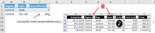
We can remove the filter table influence on the measure by wrapping it in a NONVISUAL function. This time our TotalSalesAmount is exactly 416.455.001. The image below is from PBID, as this NONVISUAL function was not introduced into Excel.

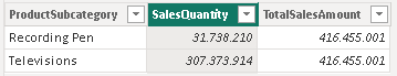
EVALUATE SUMMARIZECOLUMNS(      ProductSubcategory[ProductSubcategory]    , NONVISUAL( TREATAS( { "Recording Pen", "Televisions" }         , ProductSubcategory[ProductSubcategory] ) )    , "SalesQuantity", [TotalSalesAmount]    , "SalesAmount", CALCULATE( [TotalSalesAmount], ALLSELECTED( Sales )  ) ) ORDER BY  ProductSubcategory[ProductSubcategory]

IGNORE

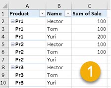
When we apply aggregations, rows where all measures are blank, will be excluded from the result.
We use VALUES function because there is no row context in the SUMMARIZECOLUMNS function.

EVALUATE SUMMARIZECOLUMNS(      ProductCategory[ProductCategory]    , "SalesQuantity", IF( VALUES(  ProductCategory[ProductCategory] ) = "TV and Video"                                    , BLANK(), SUM( Sales[SalesQuantity] ) )    , "SalesAmount", IF( VALUES(  ProductCategory[ProductCategory] ) = "TV and Video"                                   , BLANK(), SUM( Sales[SalesAmount] ) ) ) ORDER BY ProductCategory[ProductCategory]

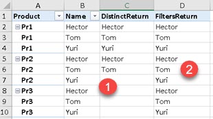
We can use the IGNORE function to treat some measures as they were blank. If some of the measures values are blank, and others are IGNORED, then such rows will not be part of a result.

EVALUATE SUMMARIZECOLUMNS(      ProductCategory[ProductCategory]    , "SalesQuantity", IF( VALUES(  ProductCategory[ProductCategory] ) = "TV and Video"                                    , BLANK(), SUM( Sales[SalesQuantity] ) )    , "SalesAmount", IGNORE( SUM( Sales[SalesAmount] ) ) ORDER BY ProductCategory[ProductCategory]

Using IGNORE on all the rows will not hide all data. Contrary, it will display all of the rows.

EVALUATE SUMMARIZECOLUMNS(      ProductCategory[ProductCategory]    , "SalesQuantity", IGNORE( SUM( Sales[SalesQuantity] ) )    , "SalesAmount", IGNORE( SUM( Sales[SalesAmount] ) ) ORDER BY ProductCategory[ProductCategory]

ROLLUPADDISSUBTOTAL

ROLLUPADDISSUBTOTAL basics

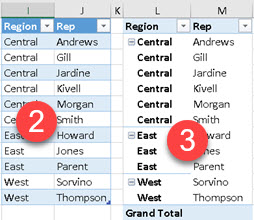
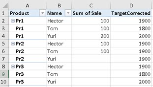
SUMMARIZECOLUMNS can have subtotals and grandtotal calculated using the ROLLUPADDISSUBTOTAL helper function. This function accepts at least two arguments. First is the column used for grouping. For the items in this column, we would get subtotals. The second argument is the name of the new column which will say TRUE or FALSE depending on whether that row is a detail row or a subtotal row.

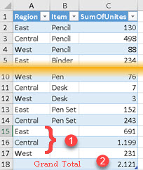
In the image bellow we can see three new rows with subtotals. There is, also, one more column that shows whether the row is a subtotal for a particular column ( TRUE or FALSE ).

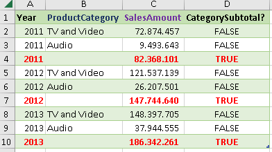
EVALUATE SUMMARIZECOLUMNS(       Calendar[Year]    ,  ROLLUPADDISSUBTOTAL( ProductCategory[ProductCategory], "CategorySubtotal?" )    , "SalesAmount", [TotalSalesAmount] ) ORDER BY  Calendar[Year] ASC                 , ProductSubcategory[ProductSubcategory] DESC

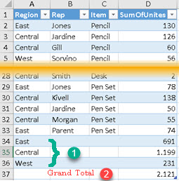
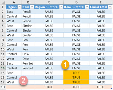
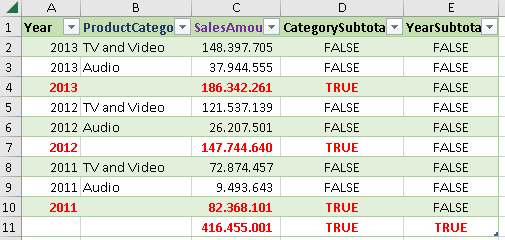
This happens if we wrap each grouping column with ROLLAPADDISSUBTOTAL. We get all possible subtotals.

EVALUATE SUMMARIZECOLUMNS(       ROLLUPADDISSUBTOTAL( Calendar[Year], "YearSubtotal?" )    ,  ROLLUPADDISSUBTOTAL( ProductCategory[ProductCategory], "CategorySubtotal?" )    , "SalesAmount", [TotalSalesAmount] ) ORDER BY  Calendar[Year] ASC                 , ProductCategory[ProductCategory] DESC

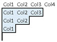
It is possible to place all the grouping columns together in a singe ROLLUPADDISSUBTOTAL function. In that case, we would get hierarchical subtotals, from left to right ( like in Excel pivot table ).

EVALUATE SUMMARIZECOLUMNS(       ROLLUPADDISSUBTOTAL( Calendar[Year], "YearSubtotal?"                                                , ProductCategory[ProductCategory], "CategorySubtotal?" )    , "SalesAmount", [TotalSalesAmount] ) ORDER BY  Calendar[Year] DESC, ProductCategory[ProductCategory] DESC

ROLLUPADDISSUBTOTAL filters

We can create a single filter table. We can place this filter table in the ROLLAPADDISSUBTOTAL function and that way we can filter our subtotals and grand total. We can place this argument at the beginning, and at the end of ROLLUPADDISSUBTOTAL function. At the start it would only filter the value of grand total. At the end, it would filter only column items.

In this example below we place it in both places. This would filter both the grand total and the items. The images are from PBID because this argument is not introduced into Excel.

VAR RollupFilter = TREATAS( { "Recording pen"}; OnlyNeeded[ProductSubcategory] ) VAR Result  = SUMMARIZECOLUMNS(       ROLLUPADDISSUBTOTAL( RollupFilter         ; OnlyNeeded[ProductSubcategory]         ; "SubcategorySubtotal?"         ; RollupFilter )    ; "SalesAmount"; [TotalSalesAmount] ) RETURN Result

This would be the results if we placed this argument only at the beginning, or only at the end of the ROLLUPADDISSUBTOTAL function.

At the beginning, it influence only grand total.

At the end, it influence only subtotals.

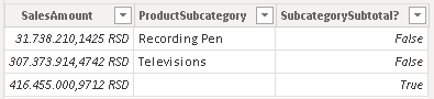
ROLLUPGROUP

By placing some columns in a ROLLUPGROUP, we will observe them together. That is why their individual subtotals will not appear in our table. If we want to exclude some subtotals, we use ROLLUPGROUP.

In this example we don't have subtotals for ProductCategory and SubCategory. They are excluded because we placed this two columns in the ROLLUPGROUP function.

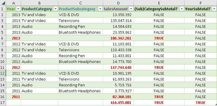
EVALUATE SUMMARIZECOLUMNS(           ROLLUPADDISSUBTOTAL(            Calendar[Year]          , "YearSubtotal?"          , ROLLUPGROUP( ProductCategory[ProductCategory]                                     , ProductSubcategory[ProductSubcategory] )          , "(Sub)CategorySubtotal?"      )      , "SalesAmount"      , [TotalSalesAmount]  ) ORDER BY  Calendar[Year] DESC                 , ProductCategory[ProductCategory] DESC                 , ProductSubcategory[ProductSubcategory] DESC

Sample file can be downloaded from here:

Requirement

We have a table like (1). This tables shows how many units of product has been sold on each date in each region. We want to get pivot table (2) that shows how many days, sale was bigger than 75, 53 or 27 units. We want to observe those values per year so we added a slicer for years (3).

Needed calculations

If our data is (1), first we need to group our data by Region and OrderDate and to calculate sum of units for each group (2). That table we have to filter for values bigger than 75 (3). Then, again, we have to do grouping by Region and to count rows from our filtered table (4). We also have to repeat this for values 53 and 27.

Slow solution

For this calculation we could create three measures that look like the one bellow. If we have a lot of data, after clicking on slicer we would have to wait a lot for calculation to finish. Not only we do have a lot of data, but we also have demanding calculation for each measure, and we have three such measures.

MeasureOver75:=
VAR GroupByRegionOrderDate = GROUPBY( SampleTable; [Region]; [OrderDate]; "SumOfUnits"; SUMX( CURRENTGROUP(); [Units] ) )
VAR FilterOver75AndCount = COUNTROWS( FILTER( GroupByRegionOrderDate; [SumOfUnits] >= 75 ) )
RETURN FilterOver75AndCount

All three measures starts with the same step ( "GroupByRegionOrderDate" ). This step is very expensive because it is the one doing most of calculations. This step returns table. If we could just do this step once instead of repeating it for each measure, that would be great. We could make a basic measure that returns such table (1), and then three other measures that would use that table to calculate final scalar values (2).

Unfortunately, measures can not return table. They can only return scalar.

Better solution

Better solution is to create one measure that returns all three values. We can simply concatenate three numbers in one string ( "25-32-36" ). That would be result of our Basic measure. Then we can create three measures that would extract separate values. This could be our Basic measure code:

BasicMeasureString:=
VAR GroupByRegionOrderDate = GROUPBY( SampleTable; [Region]; [OrderDate]; "SumOfUnits"; SUMX( CURRENTGROUP(); [Units] ) )
VAR BiggerThen75 = COUNTROWS( FILTER( GroupByRegionOrderDate; [SumOfUnits] >= 75 ) )
VAR BiggerThen53 = COUNTROWS( FILTER( GroupByRegionOrderDate; [SumOfUnits] >= 53 ) )
VAR BiggerThen27 = COUNTROWS( FILTER( GroupByRegionOrderDate; [SumOfUnits] >= 27 ) )
VAR Result = BiggerThen75 & "-" & BiggerThen53 & "-" & BiggerThen27
RETURN Result           

It would return string „25-32-36". Then we can use three additional measures to extract three separate values:

FirstPartOfString:=VALUE( LEFT( [BasicMeasureString]; 2 ) )             //returns 25
MiddlePartOfString:=VALUE( MID( [BasicMeasureString]; 4; 2 ) )    //returns 32
LastPartOfString:=VALUE( MID( [BasicMeasureString]; 7; 2) )          //returns 36

As we see, we only do step „GroupByRegionOrderDate" once. This way we make our calculation much faster. If our final results are numbers, we could get results even faster by using mathematical calculations to extract our values, instead of doing string manipulations. In our Basic measure we could combine three values into one value like this:

VAR Result = BiggerThen75 * 10000 + BiggerThen53 * 100 + BiggerThen27  //returns 253236

Then, we can extract separate numbers by using INT and MOD functions like this:

Dates with sale over75 := INT( [BasicMeasure] / 10000 ) //returns 25
Dates with sale over53 := INT( MOD( [BasicMeasure]; 10000 ) / 100 ) //returns 32
Dates with sale over27 := MOD( [BasicMeasure]; 100 ) //returns 36

Solution with math calculations would be significantly faster.

Sample file can be downloaded here:

Sometimes different users want pivot table sorted in different ways. If column has full names of people, it is possible to sort column either by using first names or by using last names. An additional requirement is the ability to change the sort order using a slicer.

In the example bellow, we can see that our pivot table can be sorted by "Points" (1), but two other possible sorting orders are by "Last Name" (2) or by "First Name" (3). We will create solution only for this three specific sorting methods. Points will be sorted from highest to lowest, and first and last names will be sorted alphabetically.

Helper Tables

First we have to create table in Power Pivot that will hold values for our slicer (1). We will call this table "SlicerValues".

Second, we have to create table in Power Pivot, that will have columns with sort order for every row (1). We need two such columns, one for last names and one for first names. This table will have name "SortOrdersTable".

General Idea

We know that it is possible to sort some column, in pivot table, by using some other column as sort order. First we have to right click on column which we want to sort, and then we go to Sort > More Sort Options (1). New dialog will open. In this dialog we will select "Descending (A to Z) by:" and then we will choose which column will define our sort order. In the image bellow, we decided that "Sum of Points" column (2) in DESC order is used for sorting. Now, "Full Name" column (3) is not sorted alphabetically, but according to "Sum of Points" column.

We can use mechanism, explained above, to control column "Full Name" sorting order. Idea is to create a measure, with a name "SortMeasure", that will be added to our pivot table (1). This measure values will change according to selection in the slicer (3,4,5). Our column "Full Name" will be set to sort by order defined by "SortMeasure" (2).

Now, when the user selects "First Names" (3), "Last Names" (4) or "Points" (5) in the slicer, column "SortMeasure" values will change (1) and that will sort our column "Full Name" (2). We can see in (3) that column "Full Name" is sorted by first name, in (4) by last name, and in (5) by points. At the end, column "SortMeasure" will be hidden from the user by hiding the whole spreadsheet column.

Creative process

First we have to make relation between "Full Name" columns in "SortOrdersTable" and "Data" table (1). "Data" table is the name of a table which is the base for our pivot (with "Full Name" and "Points" columns). Relation has to be "1:N" in direction "Data" to "SortOrdersTable" (2). This means that in relation dialog "Data" table has to be at the bottom. "Data" table can filter "SortOrdersTable".

Next step is to create our measure. This measure has to be reactive to slicer selection. ALLSELECTED function will return values selected in slicer as a column. With green part of code we will check whether specific individual values in slicer are part of that column. If they are, that means that those terms are selected and we will return TRUE(), otherwise we will return FALSE(). At the end, we will use SWITCH function to decide what values the measure should return. SWITCH function will return values for the first variable ( FirstNamesSelected, LastNamesSelected, PointSelected ) that returns TRUE(). For example, if FirstNamesSelected is FALSE(), and LastNamesSelected is TRUE(), values from "Last Name order" column will be returned. Those are the values that will be used to sort "Full Name" column.

SortMeasure:=
VAR FirstNamesSelected = IF( "First Names" IN ALLSELECTED( SlicerValues[SortBy] ); TRUE(); FALSE() )
VAR LastNamesSelected = IF( "Last Names" IN ALLSELECTED( SlicerValues[SortBy] ); TRUE(); FALSE() )
VAR PointsSelected = IF( "Points" IN ALLSELECTED( SlicerValues[SortBy] ); TRUE(); FALSE() )
VAR Result = SWITCH( TRUE(); FirstNamesSelected; SUM( SortOrdersTable[First Name order] ) 
                           ; LastNamesSelected; SUM( SortOrdersTable[Last Name order] )
                           ; PointsSelected; 10000 - SUM( Data[Points] ))
RETURN Result

All columns with possible result ( "First Name order", "Last Name order", "Points" ) are just wrapped in SUM function, but "Points" column has one more detail. In our measure we will transform all "Points" values into "10000 – Points". This is because, we want ascending sorting for "First Name order" and "Last Name order", but descending sorting for "Points". Because pivot table can only be in ascending or descending order at once, we need this transformation so that ascending ordering of our measure will always correctly sort our pivot table. Values of "Points" and "10000 – Points" are inversely correlated, and this solves our problem.

Descending sorting of "Points" is the same as ascending sorting of a transformation "10000 – Points".

Result

Bellow we can see our results and we can observe a few details. Columns "C" and "G" are hidden (1). This is how we will hide our "SortMeasure" column from the user. In green pivot table (2) we can see that while "SortMeasure" column is in ascending order, important column "Sum of Points" is actually in descending order, as per requirement.

In blue and orange pivot tables, there are two values selected in each slicer (3). It is not possible to force single selection in slicer in Excel without resorting to VBA. To solve this problem, we made our measure so that the first selected value is the one determining sorting order. That is why both blue and orange pivot tables are sorted by "First Names", that is the first value selected in their slicers.

Sample table can be downloaded from here: