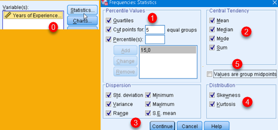
Remember and Reset the Cursor Position
What Problem Are We Solving?
When making video tutorials, it's easiest to make short videos, but sometimes we need more time to explain a topic. Even then, we can break our entire tutorial into smaller videos. Then we have a problem how to connect those small videos into a whole. This problem can be solved by placing a slide between each smaller video. If slides are not a suitable solution then we have to find a way to seamlessly connect our smaller videos. This leads us to our problem, how to record cursor position in the previous video, so that we can start recording new video with the cursor at the same position.
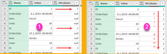
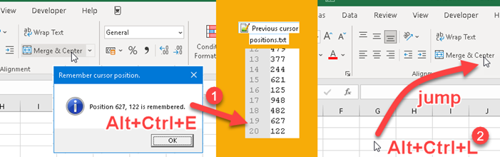
Idea is to save location of our cursor in TXT file, when some shortcut is pressed (1). This is something we have to do at the end of recording. Before we start recording the next video, using another shortcut, we would return the cursor to the last position (2). Note that the TXT file always retains the last 20 recorded positions.
I will show you a solution that doesn't use third-party software and can be use on any computer.
Recording the Last Position of the Cursor
We can record the last cursor position with a Powershell script. This script will read the current cursor position and then it will write that cursor position into TXT file.
Add-Type -AssemblyName System.Windows.Forms

$p = [System.Windows.Forms.Cursor]::Position
$X = $p.X
$Y = $p.Y

Add-Content -Path "C:\Users\Sima\Desktop\Resursi\Kursor pozicija\Previous cursor positions.txt" -Value ( $X.ToString() + "`r`n" + $Y.ToString() )

Add-Type -AssemblyName PresentationCore,PresentationFramework
$ButtonType = [System.Windows.MessageBoxButton]::OK
$MessageboxTitle = "Remember cursor position."
$Messageboxbody = "Position $X, $Y is remembered."
$MessageIcon = [System.Windows.MessageBoxImage]::Information
[System.Windows.MessageBox]::Show($Messageboxbody,$MessageboxTitle,$ButtonType,$messageicon)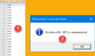 | That TXT file will keep the last 20 positions (1) so we don't have to worry about overwriting the cursor position we saved earlier. In the end we will get a message box (2) with the position of our cursor expressed in pixels. |
Resetting of the Cursor Position
Again, we'll use Powershell to reset the cursor position. First we will read the last two numbers from our TXT file. Next, we'll set the cursor position to the new location. Finally, we need to make sure that there are only the last 20 positions saved in our TXT file. We will achieve this by measuring how many lines there are in our file, and if that number is greater than 20 then we will overwrite our file with only the last 20 positions.
$file = "C:\Users\Sima\Desktop\Resursi\Kursor pozicija\Previous cursor positions.txt"
$file_data = Get-Content -tail 2 $file

Add-Type -AssemblyName System.Windows.Forms

$p = [System.Windows.Forms.Cursor]::Position
$p.X = $file_data[0]
$p.Y = $file_data[1]
[System.Windows.Forms.Cursor]::Position = $p

$content = Get-Content $file
$numberOfLines = $content.Length
if ( $numberOfLines -gt 20 )
{
  $content[($numberOfLines-20)..$numberOfLines]|Out-File $file -Force
}
Embedding Powershell Scripts into VBS Scripts
Running Powershell PS1 scripts is restricted due to security. Instead of calling our scripts directly, we'll wrap them in VBS scripts. Our code for the first and second scripts will now look like this. At the beginning and end, we need to create and destroy the shell object. We use that object to run our scripts using powershell.exe. The quotes and double quotes in the original Powershell scripts have been modified so that the script can be embedded inside a VBS script.
RECORD:
Set WshShell = CreateObject("WScript.Shell")
WshShell.Run "C:\Windows\System32\WindowsPowerShell\v1.0\powershell.exe -ExecutionPolicy Bypass -Command ""Add-Type -AssemblyName System.Windows.Forms;$p = [System.Windows.Forms.Cursor]::Position;$X = $p.X;$Y = $p.Y;Add-Content -Path 'C:\Users\Sima\Desktop\Pamcenje kursor pozicije\Previous cursor positions.txt' -Value ( $X.ToString() + """"""`r`n"""""" + $Y.ToString()  );Add-Type -AssemblyName PresentationCore,PresentationFramework;$ButtonType = [System.Windows.MessageBoxButton]::OK;$MessageboxTitle = 'Remember cursor position.';$Messageboxbody = """"""Position $X, $Y is remembered."""""";$MessageIcon = [System.Windows.MessageBoxImage]::Information;[System.Windows.MessageBox]::Show($Messageboxbody,$MessageboxTitle,$ButtonType,$messageicon)"" ", 0
Set WshShell = Nothing

RESET:
Set WshShell = CreateObject("WScript.Shell")
WshShell.Run "C:\Windows\System32\WindowsPowerShell\v1.0\powershell.exe -ExecutionPolicy Bypass -Command ""$file = 'C:\Users\Sima\Desktop\Pamcenje kursor pozicije\Previous cursor positions.txt'; $file_data = Get-Content -tail 2 $file; Add-Type -AssemblyName System.Windows.Forms;$p = [System.Windows.Forms.Cursor]::Position; $p.X = $file_data[0]; $p.Y = $file_data[1]; [System.Windows.Forms.Cursor]::Position = $p; $content = Get-Content $file; $numberOfLines = $content.Length; if ( $numberOfLines -gt 20 ) { $content[($numberOfLines-20)..$numberOfLines]|Out-File $file -Force }"" ", 0
Set WshShell = Nothing
Notice that WshShell.Run has a second argument. That argument is zero. This is used to prevent opening of a terminal window while scripts are executing.
Calling our Scripts
We need to call our scripts with keyboard shortcuts. We have to use shortcuts because we can't use the mouse for that. Our cursor must be stationary.
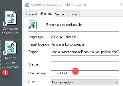 | We can create global shortcuts by creating two shortcut files that target our VBS scripts (1). These two shortcut files must be placed on the desktop, otherwise the keyboard shortcuts will not work. Next we need to go to the properties of our shortcut files and there on the "Shortcut" tab we can set the keys (2) that will be used to call our VBS scripts. |
Sample files can be downloaded below. Remember to change fullpath of "Previous cursor positions.txt" file inside of each VBS script. Also, change the target of each shortcut file. Change fullpath of powershell executive file, too.