All tables in the same schema must have unique names. Tables cannot have the same name as a view. When we create a new table, we can omit the schema name. In this case, the table will be created in the current schema.
This is the simplest CREATE TABLE statement. We need to specify table name, column name and column data type. CREATE TABLE Tab1 ( Col1CLOB );
If we try to create a table with the same name again, we will get an error. CREATE TABLE: name 'tab1' already in use
We can avoid that error with clause "IF NOT EXISTS". A new table will only be created if no other table with that name exists. If a table with that name already exists, nothing will happen, but we won't get an error. CREATE TABLE IF NOT EXISTS Tab1 ( Col1 CLOB );
If we want to create a table in a non-current schema, we must use the fully qualified table name. Of course, we have to have enough privileges for that. CREATE TABLE sys.Tab1 ( Col1 CLOB );
After the data type we can include some options that better describe our column. Those options are DEFAULT, NOT NULL, PRIMARY KEY, UNIQUE.
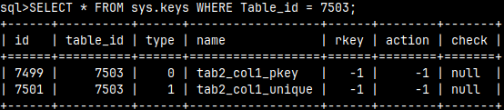
In the system table sys.keys, we can now find our constraints for the primary key and for the unique constraint. Both of these constraints belong to table Tab2, which has ID 7503. SELECT * FROM sys.keys WHERE Table_id = 7503;
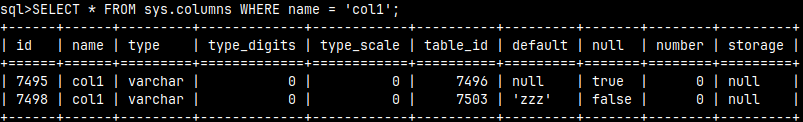
There is also a system table sys.columns where we can find columns named "col1". The column in the last row belongs to table Tab2, because table_id = 7503. SELECT * FROM sys.columns WHERE name = 'col1';
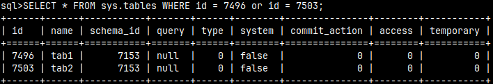
If we read from the table sys.tables, we can search for our tables by using their ID-s. SELECT * FROM sys.tables WHERE id = 7496 or id = 7503;
It is possible to insert nothing into our table. Such a statement will work. When we try to read from our table, we will see that the DEFAULT value has been written into it.
If we try to write a NULL value to our table, such an act will fail, because our column is defined as a NOT NULL column. INSERT INTO Tab2 VALUES (null);
If we try to write the default value again to our table, it will fail. We cannot have two rows with the same value in column Col1, due to primary key constraints.
In the real world, we would never mix DEFAULT and PRIMARY KEY constraints. PRIMARY KEY means that each row should be unique. That's the opposite of what DEFAULT is trying to do. PRIMARY KEY also means that our column does not accept nulls, so there is no need for a formal NOT NULL constraint. UNIQUE is also redundant as PRIMARY KEY will not allow duplicates anyway. In the real world, we would never use all the constraints on the same column.
Creating a Table Based on Some Other Table
Using LIKE operator
Previously, we created a table Tab2 with a column Col1 that has many constraints. Now we want to create a new table that will be a copy of Tab2, but will have a few more columns. We can do it in one step. This statement below will create all the columns found in the Tab2 table and place them in the Tab3 table. Tab3 will also have another column of type INTEGER.
CREATE TABLE Tab3 ( LIKE Tab2, Col2 INTEGER ); We can see on the image, Tab3 inherited "Col1" from the table Tab2. We also added one more column "Col2" in table Tab3.
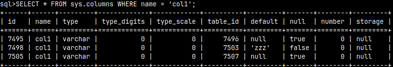
Constraints on columns in Tab2 will not be inherited. If we read from system table sys.columns, we will notice that table with ID 7507 (Tab3), doesn't have the same constraints as the table 7503 (Tab2). All of the constraints are lost.
Using AS SELECT
By using AS SELECT statement we would create a table based on some SELECT query. We can type:
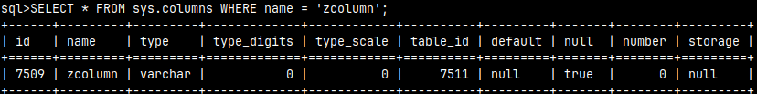
CREATE TABLE Tab5 ( Zcolumn, Today )
AS ( SELECT Col1, current_date  FROM Tab2 );
The new table will not inherit the constraints from the old column. We can see that we don't have the same restrictions on the 'zcolumn' column as we did on the 'col1' column.
We don't have to provide aliases. We can use original column names. CREATE TABLE Tab6 AS ( SELECT Col1, current_date AS Today FROM Tab2 );
If add "WITH NO DATA" clause, then we would get the columns, but without data. CREATE TABLE Tab7 AS ( SELECT Col1, current_date AS Today FROM Tab2 ) WITH NO DATA;
Table Constraints
We can place PRIMARY KEY constraint on one column. It won't help us if our table has a composite primary key. If this is the case, we need to place constraints on the table itself. We can write the statement like this:
URL Data Type is used for storing URL addresses. We will create a table with this type of data. We can also use something like URL(512) if we want to limit the number of characters.
CREATE TABLE URLtable( URLcolumn URL );
Inside of this column we can store both string and URL data types.
INSERT INTO URLtable ( URLcolumn ) VALUES ( 'https://www.monetdb.org/documentation/user-guide/' );
INSERT INTO URLtable ( URLcolumn ) VALUES ( URL'https://www.monetdb.org/documentation/user-guide/' );
We can create URL data type by using CONVERT and CAST functions, or by using URL prefix:
SELECT CONVERT('https://www.monetdb.org/documentation/user-guide/', url);
SELECT CAST('https://www.monetdb.org/documentation/user-guide/' AS url);
SELECT URL 'https://www.monetdb.org/documentation/user-guide/';
We can then read all these parts using the MonetDB URL functions. If a part does not exist, these functions will return NULL. All functions return a CLOB.
To extract the "host" we have two functions, GETHOST and URL_EXTRACT_HOST. The URL_EXTRACT_HOST function accepts a second argument that can exclude the "www" part from the host, if the value of this argument is true.
SELECT SYS.GETPROTOCOL( URLcolumn ) FROM URLtable;
https
SELECT SYS.GETUSER(URLcolumn) FROM URLtable;
me
SELECT SYS.GETHOST( URLcolumn ) FROM URLtable; SELECT SYS.URL_EXTRACT_HOST( URLcolumn, false)FROM URLtable; SELECT SYS.URL_EXTRACT_HOST( URLcolumn, true ) FROM URLtable;
www.monetdb.org www.monetdb.org monetdb.org
SELECT SYS.GETPORT( URLcolumn ) FROM URLtable;
458
SELECT SYS.GETCONTEXT( URLcolumn ) FROM URLtable;
/Doc/Abc.html
SELECT SYS.GETQUERY( URLcolumn ) FROM URLtable;
lang=nl&sort=asc
SELECT SYS.GETANCHOR( URLcolumn ) FROM URLtable;
example
The path (context) can be further divided into:
SELECT SYS.GETFILE( URLcolumn ) FROM URLtable;
Abc.html
SELECT SYS.GETBASENAME( URLcolumn ) FROM URLtable;
Abc
SELECT SYS.GETEXTENSION( URLcolumn ) FROM URLtable;
html
From the host we can read the domain separately:
SELECT SYS.GETDOMAIN( URLcolumn ) FROM URLtable;
org
Using the SIS.ISAURL function, we can check if something is a valid URL.
SELECT SYS.ISAURL( URLcolumn ) FROM URLtable;
true
Robots.txt is a text file with instructions for search engines (e.g. Google). It is always located in the root directory of the web server. This function will return the location of Robots.txt.
SELECT SYS.GETROBOTURL( URLcolumn ) FROM URLtable;
https://me@www.monetdb.org:458/robots.txt
All the functions above will accept either string or URL data type as its argument. For creation of a new URL, we need arguments that are strings (or integer for ports). Function for creation of a new URL-s, can accept two combinations of arguments, as we can see bellow. Compound argument 'usr@www.a.com:123' is called "authority".
This data type is used to store IPv4 addresses, such as '192.168.1.5/24'. We can create column with this data type, and we can write strings and network data type in this column.
For creation of INET data type we can use CONVERT, CAST functions or INET prefix operator.
SELECT CONVERT('192.168.1.5/24', INET);
SELECT CAST('192.168.1.5/24'  AS INET);
SELECT INET '192.168.1.5/24';
Network Data Type Operators
Network data type operators are used to compare two network addresses. Network addresses consist of four numbers between 1 and 255 ( 1.1.1.1 to 255.255.255.255 ). We can add zeros to those numbers, so that each number has three digits. Then we can remove dots.
17.18.203.1 =>
017.018.203.001 =>
017018203001
221.42.2.56 =>
221.042.002.056 =>
221042002056
Logic of comparison is simple, if 221042002056 > 017018203001 then 221.42.2.56 > 17.18.203.1 . We can test this with MonetDB operator.
SELECT INET '221.42.2.56' > INET '17.18.203.1';
true
We can use all mathematical operators. If they can work on numbers, they can work on network addresses.
<
<=
=
>=
>
<>
Network Data Type Operators for Belonging
Maximal network address can be 255.255.255.255. Number 255 can be presented as 28. This means that total number of combinations is 28 x 28 x 28 x 28=232. We can say that each number has 8 bits, but total IP address has 32 bits.
We have address for a network, and address for a computer on that network.
Network address
Computer address
221
221.42.2.56
On large networks we can have many computers, so we need three numbers to label them all.
221.42
221.42.2.56
On medium networks two numbers are enough to mark all of our computers.
221.42.2
221.42.2.56
On small networks we only need one number. Here we can have up to 255 computers.
In the second column, in the table above, we see that the computer address is composed of two parts. One part will indicate the network and the other will be for the computer on that network. I used red and black to make a difference. In the real world, this distinction is made using this syntax such as "221.42.2.56/24". This "/24" suffix means that the first 24 bits (the first three numbers) are for the network and the rest for the computer.
Now we can understand operators for belonging. These operators will tell us whether some computer address belong to some network.
SELECT INET '192.168.1.5' << INET '192.168.1/24';
true
Computer 192.168.1.5 belongs to network 192.168.1.
Same as above, but this will also return trueif we compare two same networks. In our example we have the same network on the both side of the operator.
Of course, we can also use reverse operators >> and >>=, so we have to be careful what is on the left, and what is on the right side of our operator.
Network Data Type Functions
All of these functions will accept only INET data type.
SELECT SYS.ABBREV( INET '10.1.0.0/16');
10.1/16
This function will remove the trailing zeros, to shorten network address. Returns CLOB.
SELECT SYS.BROADCAST( INET '192.168.1.5/24');
192.168.1.255/24
If we want to send message to all of the computers on the network, we use broadcast address. This is network part of address, and all other numbers are 255. In our example we have 192.168.1 + 255 = 192.168.1.255. Returns INET.
SELECT SYS.HOST( INET '192.168.1.5/24');
192.168.1.5
This will just extract host from network address (by removing "/24"). Returns CLOB.
Returns INET with "/24" changed to "/16". The second argument is an INTEGER.
SELECT SYS.TEXT( INET '192.168.1.5' );
"192.168.1.5/32"
Returns INET as a text. It attached "/32" part.
There is another function. I don't know what it's used for, but I figured out how it works. It seems that this function will show us the maximum number of computers that can be in this network.
SELECT SYS.HOSTMASK( INET '192.168.23.20/30' );
0.0.0.3
It is calculated like 232 / 230 = 22 = 4. Result is 4 -1 = 3.
SELECT SYS.HOSTMASK( INET '192.168.23.20/24' );
0.0.0.255
It is calculated like 232 / 224 = 28 = 256. Result is 256 – 1 = 255.
SELECT SYS.HOSTMASK( INET '192.168.23.20/17' );
0.0.127.255
It is calculated like 232 / 217 = 215 = 27 x 28 = 128 x 256. Result is 128 -1 = 127 and 256-1=255.
We have some JSON data. We can create a column that would accept string data type and put this JSON inside. If we want more functionality, we can use special JSON data type. In that case only valid JSON could be placed into that column.
We create a JSON column like this. Data type could be JSON, or JSON(100) if we want to limit length.
We can read from JSON column like from any column with "SELECT * FROM JsonTable;", but if we want to get only some part of JSON code, we have to use JSONpath expressions. JSONpath expressions can define what part of JSON code we want to read. JSONpath expression should be placed as argument in JSON.FILTER function. Result will always be returned inside square brackets. Result is also of JSON data type. JSONpath expressions are case sensitive.
SELECT JSON.FILTER( JsonColumn, '$') FROM JsonTable;
[--this will return the whole json string--]
$ represents root of a JSON.
SELECT JSON.FILTER( JsonColumn, '$.store.bicycle.color') FROM JsonTable;
["red"]
We read the direct child of the hierarchical path.
SELECT JSON.FILTER( JsonColumn, '$..Title') FROM JsonTable;
["Door","Sword"]
SELECT JSON.FILTER( JsonColumn, '$.store..color') FROM JsonTable;
["red"]
This will return all elements that are of type "title" regardless of where they are in the hierarchy. We can limit this type of filter to the interior of the "store" only.
There are other functions for use with JSON, that do not use JSONpath.
SELECT JSON.TEXT(JsonColumn, '_|_' )  FROM JsonTable;
Door_|_8.95_|_Sword_|_12.99_|_red_|_19.95_Runako
This will collect all the values from our JSON. The values will be concatenated with a separator string between them. If we don't provide second argument, the separator will be a space character.
All of these functions will return the number four as DOUBLE. There is also a function that accepts the same arguments but will return an INTEGER . Both functions will return NULL if fail. JSON."INTEGER"( JSON '{"n":4}' )
This function will return "true" if it is a JSON object. If it is a JSON array, then it will return false. This function also accepts STRING data type. SELECT JSON.ISOBJECT( '{"n":4}');
SELECT JSON.ISARRAY( JSON '[4]' ); true
This function returns true when JSON is an array (it also accepts a STRING data type).
SELECT JSON.ISVALID( JsonColumn ) FROM JsonTable; true
This function will return "true" if the given JSON code is valid.
SELECT JSON.LENGTH( JsonColumn ) FROM JsonTable; 2
This will count the top elements in our JSON.
SELECT JSON.KEYARRAY( JsonColumn ) FROM JsonTable;["store","employee"]
This function will return all the top keys from the JSON sample. The top-level JSON must be an object, otherwise an error will be returned.
A UUID is a unique value created by an algorithm. The UUID looks like this "65950c76-a2f6-4543-660a-b849cf5f2453". The UUID is represented as 32 hexadecimal digits separated into 5 groups of digits. The first group has 8 digits, then we have three groups of 4 digits, and finally there is one group of 12 digits. Together they define a really big number. Every time we call a function to create a new UUID, it will likely create a new value that was never used, anywhere in the world. Such values are used as a synthetic key that is globally unique.
We can create a new UUID value with this function:
SELECT SYS.UUID() AS UUID; 65950c76-a2f6-4543-660a-b849cf5f2453
If we want to check whether some value is a valid UUID we can use function SYS.ISAUUID( string ). This function will return TRUE if we have a string formatted like 65950c76–a2f6–4543–660a–b849cf5f2453 or like 65950c76a2f64543660ab849cf5f2453, without hyphens.
We can transform a string into a UUID data type using the CAST or CONVERT functions, or we can use the UUID unary operator:
select cast( '26d7a80b-7538-4682-a49a-9d0f9676b765' as uuid) as uuid_val;
select convert('83886744-d558-4e41-a361-a40b2765455b', uuid) as uuid_val;
select uuid 'AC6E4E8C-81B5-41B5-82DE-9C837C23B40A' as uuid_val;
In a table, synthetic (surrogate) key is a column which have a unique value for each row, but its content is not derived from application data, but is generated. If none of the rows is deleted from this table, then this column will usually have numbers as a sequence 1,2,3,4…
Synthetic key
ID number
Name
1
E02387
Netsai
2
E04105
Amos
3
E02572
Taurai
4
E02832
Mischeck
There are many advantages in using surrogate keys but this time we will talk only about that how to create them in MonetDB. We can use code like this:
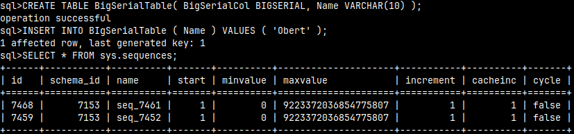
CREATE TABLE SerialTable ( SerialCol SERIAL, Name VARCHAR(10) );
When we enter data in this column, we do not specify values for SerialCol. Those values will be automatically created because this column is of SERIAL data type.
INSERT INTO SerialTable (Name) VALUES ('Obert');
When we read from this table, this would be the result. Number one will be automatically added to SerialCol.
SerialCol
Name
1
Obert
If we repeat this INSERT statement several time, each time we would get next number.
SerialCol
Name
1
Obert
2
Obert
3
Obert
This means that, for this column, there is a database object that is remembering last used number, so that next time it can provide next number in a sequence. We can find that database object in sys.sequences system table. Although this table claims that maxvalue is some huge number ( upper limit for BIGINT, or 9223372036854775807 ), this column will actually be of the type INTEGER. Starting value is one, and increment is also one. That is why we are getting numbers 1,2,3…
It is also possible to use BIGSERIAL instead of the SERIAL. In that case our column would be really of the type BIGINT.
If we want to define what kind of integer to use then we are using syntax like this. Instead of INT we can use any other integer data type like TINYINT, SMALLINT, BIGINT, HUGEINT.
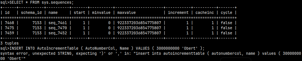
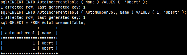
CREATE TABLE AutoIncrementTable ( AutoNumberCol INT AUTO_INCREMENT, Name VARCHAR(10) );
In that case "sys.sequences" table will still show that maxvalue is upper limit for BIGINT, but the real limit will be for INTEGER data type. If we try to enter a value for AutoNumberCol by ourselves, that activity will fail if the number is bigger than 2.7 billion which is upper limit for INTEGER data type.
Maxvalue is always set to BIGINT upper limit because internally MonetDB is storing serial numbers as BIGINT. This doesn't mean that you can not use HUGEINT as AUTO_INCREMENT, you can.
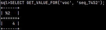
We can generate a new value for our sequence with this statement. "seq_7452" is the name of our sequence. This will increment our sequence by one, so this statement should be used to get next number and then to use it for something. This is usually useful when we want to create new value, and then to use it both in primary key column and foreign key column.
SELECT NEXT VALUE FOR seq_7452;
When we are using SERIAL or BIGSERIAL data type, that column will get PRIMARY KEY and NOT NULL constraints.
Values Entered by the User
Whenever we use SERIAL, BIGSERIAL, we still have ability to enter sequence values by ourselves. If we try to insert a number that already exists in the table it will raise primary key exception.
This is not true if we use AUTO_INCREMENT syntax. In that case we don't have primary key constraint, so it will not be a problem if we enter two same values in our AUTO_INCREMENT column.
If we want to disable ability to enter our own value in sequence column, then we could use this generic syntax. THIS SYNTAX WILL NOT WORK IN MONETDB. It will create a new sequence, but it will not prevent us from entering our own values.
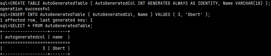
CREATE TABLE AutoGeneratedTable ( AutoGeneratedCol INT GENERATED ALWAYS AS IDENTITY, Name VARCHAR(10) )
This web page explains that this should not be allowed, but in MonetDB it doesn't work as it should.
[Err] ERROR:  cannot insert into column "rank_id"
DETAIL:  Column "rank_id" is an identity column defined as GENERATED ALWAYS.
https://www.sqltutorial.org/sql-identity/
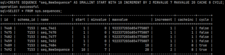
Sequence parameters
Although previous syntax is not prohibiting from entering our own values, that syntax will allows us to use sequence parameters.
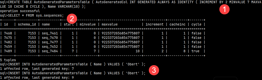
CREATE TABLE AutoGeneratedParametersTable ( AutoGeneratedCol INT GENERATED ALWAYS AS IDENTITY ( INCREMENT BY 2 MINVALUE 7 MAXVALUE 10 CACHE 8 CYCLE ), Name VARCHAR(10) );
The parameters (1), allow us to control what will be the content of sys.sequences table (2). As we can see, now the first sequence number will be 7 and next sequence number will be 9 (3).
We can use these parameters:
START WITH number– This is the starting number in sequence. It could be negative or positive. If this parameter is not declared, then the default value is MINVALUE for ascending sequences and MAXVALUE for descending sequences. START WITH parameter must be bigger than MINVALUE parameter.
INCREMENT BY number – This way we define difference between two consecutive numbers in a sequence. Default value is 1. If "number" is positive then we have ascending sequence. For negative "number", sequence will be descending.
NO MINVALUE – NO MIN VALUE means that we are using default value. Default value for ascending sequences is either 1 or START WITH parameter. Default value for descending sequences is minimum value for data type that is associated with the sequence.
MINVALUE number – Can be negative or positive. Must be smaller than MAXVALUE.
NO MAXVALUE – This means that we are using the default value. For ascending sequences that value will be the maximum value of the data type that is associated with the sequence. For descending sequences, it is either -1 or START WITH number.
MAXVALUE number – Can be positive or negative number. Must be greater than minimum value.
NO CACHE – System will cache next number to be used. This could create problem because in the case of the system failure, that number will be lost. We can prevent such scenario with NO CACHE.
CACHE number–In order to increase performance, we can cache several next values for our sequence. Number of cached values will be smaller or equal to the CACHE number. In the case of the system failure, all these values will be lost.
CYCLE – After ascending sequence reach the end of a range, it will start again from the minimal value for associated data type or from the MINVALUE parameter. After descending sequence reach the start of a range, it will start again from the maximal value for associated data type or from the MAXVALUE parameter.
NO CYCLE – This will not allow looping. If we reach the value outside of the limits of our range, an error will be raised.
Sequence as an Object
We can create sequence as an object and then we can use that object when we create a new table. We create a new sequence like this. We can define all of the parameters in this statement.
CREATE SEQUENCE "seq_NewSequence" AS SMALLINT START WITH 10 INCREMENT BY 2 MINVALUE 7 MAXVALUE 20 CACHE 8 CYCLE;
Now that we have our sequence, we can use it for our new table. We will bind sequence object to our column as a default value.
CREATE TABLE SequenceObject ( SequenceCol SMALLINT DEFAULT NEXT VALUE FOR "seq_NewSequence", name VARCHAR(10) );
If we want to alter our sequence object, then we use this statement. Again, we can use all of the parameters. The only difference is that here instead of "START WITH" we use "RESTART WITH".
ALTER SEQUENCE "seq_NewSequence" RESTART WITH 21 INCREMENT BY 3 MINVALUE 15 MAXVALUE 100 CACHE 10 NO CYCLE;
Sequence object can be deleted with this statement. It is only possible to delete sequence object if references to that object are deleted. That means that we have to change DEFAULT value of a columns that are using that sequence object.
DROP SEQUENCE "seq_NewSequence";
Info functions
Two statements below are the same:
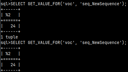
SELECT NEXT VALUE FOR seq_NewSequence;
SELECT NEXT_VALUE_FOR( 'voc', 'seq_NewSequence' );
Both of them will return number 21, but the next time we call them they will return number 22. They shift the sequence.
If we just want to check what is the next number in a sequence then we can use this function. As we can see, it will always return the same number, sequence will not be shifted after each usage.
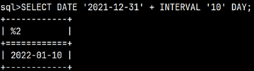
INTERVAL data types allow us to conduct arithmetic calculations with temporal data types. Keyword DATE is casting operator. This operator is used so that Monetdb transform string to date data type.
SELECT DATE '2021-12-31' + INTERVAL '10' DAY;
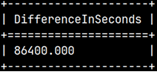
It is possible to subtract two dates or times. Result will be interval in seconds.
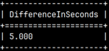
SELECT date '2020-09-28'
     - date '2020-09-27' AS "DifferenceInSeconds";
SELECT time '14:35:45'
     - time '14:35:40' AS "DifferenceInSeconds";
Current Date and Time
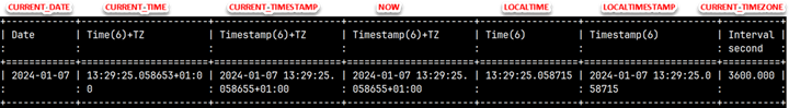
With these variables we can get information about current date, time and time zone (TZ).
SELECT CURRENT_DATE as "Date"
     , CURRENT_TIME as "Time(6)+TZ"
     , CURRENT_TIMESTAMP as "Timestamp(6)+TZ"
     , NOW as "Timestamp(6)+TZ"
     , LOCALTIME as "Time(6)"
     , LOCALTIMESTAMP as "Timestamp(6)"
     , CURRENT_TIMEZONE as "Interval second";
Transform Strings to Temporal Data Types
There are several ways how we can create temporal data types from the strings. If we have dates, times, or timestamps in ISO format then we can use casting operator, casting function or convert function.
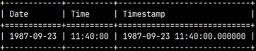
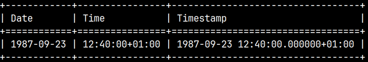
SELECT DATE '1987-09-23' AS "Date"
     , TIME '11:40' AS "Time"
     , TIMESTAMP '1987-09-23 11:40' AS "Timestamp";
—————————————————– You can also use TIMETZ, TIMESTAMPTZ.
SELECT CAST('1987-09-23' as date) AS "Date"
     , CAST('11:40' as time) AS "Time"
     , CAST('1987-09-23 11:40' as timestamp) AS "Timestamp";
SELECT CONVERT('1987-09-23', DATE) AS "Date"
     , CONVERT('11:40', TIME) AS "Time"
     , CONVERT('1987-09-23 11:40', TIMESTAMP) AS "Timestamp";
If string is not in temporal ISO format, then we have to use functions str_to_date, str_to_time or str_to_timestamp. These functions have second argument where we describe how to interpret string.
SELECT STR_TO_DATE('23-09-1987', '%d-%m-%Y') AS "Date"
     , STR_TO_TIME('11:40', '%H:%M') AS "Time"
     , STR_TO_TIMESTAMP('23-09-1987 11:40', '%d-%m-%Y %H:%M') AS "Timestamp";
Do it Reverse, Transform Dates and Times to Strings
Counterpart to functions above, are functions that transform temporal types to strings. Here we have functions DATE_TO_STR, TIME_TO_STR and TIMESTAMP_TO_STR. Again, we are using specifiers to describe how we want our string to look like.
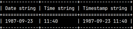
SELECT DATE_TO_STR( DATE '1987-09-23', '%Y-%m-%d') AS "Date string"
     , TIME_TO_STR( TIME '11:40', '%H:%M') AS "Time string"
     , TIMESTAMP_TO_STR( TIMESTAMP '1987-09-23 11:40', '%Y-%m-%d %H:%M') AS "Timestamp string";
Extracting Parts of Times and Dates
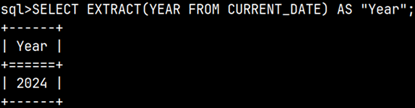
It is possible to extract parts of temporal data types by using function EXTRACT.
EXTRACT(YEAR FROM CURRENT_DATE)
We can extract these parts:
YEAR
QUARTER
MONTH
WEEK
DAY
HOUR
MINUTE
SECOND
DOY
DOW
CENTURY
DECADE
It is also possible to use specialized functions to extract temporal parts. Some of these functions have double quotes around them.
"second"(tm_or_ts)
"second"(timetz '15:35:02.002345+01:00')
2,002345
"minute"(tm_or_ts)
"minute"(timetz '15:35:02.002345+01:00')
35
"hour"(tm_or_ts)
"hour"(timetz '15:35:02.002345+01:00')
16
week(dt_or_ts)
week(date '2020-03-22')
12 >ISO week<
"month"(dt_or_ts)
"month"(date '2020-07-22')
7
quarter(dt_or_ts)
quarter(date '2020-07-22')
3
"year"(dt_or_ts)
"year"(date '2020-03-22')
2020
dayofmonth(dt_or_ts)
dayofmonth(date '2020-03-22')
22
dayofweek(dt_or_ts)
dayofweek(date '2020-03-22')
7 >Sunday<
dayofyear(dt_or_ts)
dayofyear(date '2020-03-22')
82
century(dt)
century(date '2020-03-22')
21
decade(dt_or_ts)
decade(date '2027-03-22')
202
These two functions can help to extract days or seconds from seconds interval.
"day"(sec_interval)
"day"(interval '3.23' second * (24 * 60 * 60))
3
"second"(sec_interval)
"second"(interval '24' second)
24
Max and Min Date or Time
This is how we can find latest or earliest date or time.
greatest(x, y)
greatest(date '2020-03-22', date '2020-03-25')
date '2020-03-25'
least(x, y)
least(time '15:15:15', time '16:16:16')
time '15:15:15'
Difference Between Two Timestamps – timestampdiff functions
When subtracting two timestamps we can decide in which measure units to get the result.
This is great function that allows to round our Timestamp to 'millennium', 'century', 'decade', 'year', 'quarter', 'month', 'week', 'day', 'hour', 'minute', 'second', 'milliseconds' or 'microseconds'. In example bellow we rounded our timestamp to months. That is why all the values to the right side of the month are getting their minimal values.
If we want to transform temporal data in and from Unix time, then we can use these two functions. One will transform number of seconds (counted from 01/01/1970, which is beginning of time) to regular timestamp. Second one will do the reverse. It will transform regular timestamp to seconds from the beginning of Unix time.