While typing some formula, we can click on spreadsheet cell to get its reference. If the cell is inside declared table, our reference will be structured reference.
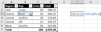
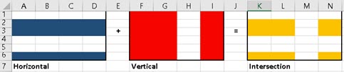
Structured reference works by cutting horizontal and vertical slices of a table, and then it returns intersection of those slices.
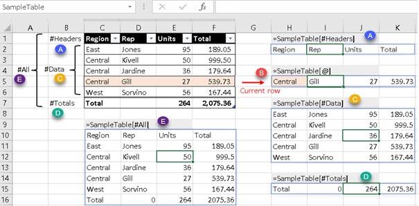
-[#Headers] returns table header (A).
-[@] returns current row (B).
-[#Data] returns table body (C).
-[#Totals] returns Total row (D).
-[#All] returns the whole table (E).
ㅤSo, when we combine name of a Table with some of specifiers, we can get horizontal slices of a table.
ㅤOne special specifier is "[@]". This specifier means that we'll get data from a row where our formula is placed. If our formula is in cell H5, then we are going to get data from cells C5:F5 in the table.
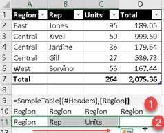
Vertical slicing can be done in two ways. We can slice only one column, and we can slice several consecutive columns.
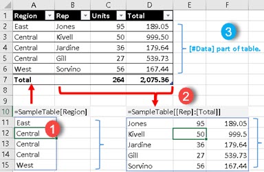
(1) is how to reference only one column.
(2) is how to reference several consecutive columns.
We can notice (3) that we don't get whole columns. We only get [#Data] part of columns. This is because [#Data] horizontal slicing is the default. If we want some other horizontal part of table, then we have to combine horizontal and vertical specifiers.
Combining specifiers
Now we have to use two specifiers. First we write horizontal specifier, and then the vertical one. Yellow example bellow, returns whole "Units" column because horizontal specifier is [#All]. Blue example returns headers for two consecutive columns because horizontal specifier is [#Headers]. Red example is different. It uses two horizontal specifiers. This way we can only use combinations ( [#Data],[#Headers] ) and ( [#Data],[#Totals] ). Red example returns "Total" column without its header. Green example assumes that formula is in the sixth row. That is why it returns values for columns "Region" and "Rep" in sixth row.
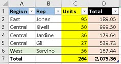
=SampleTable[[#All],[Units]]
=SampleTable[[#Headers],[Region]:[Rep]]
=SampleTable[[#Data],[#Totals],[Total]]
=SampleTable[@[Region]:[Rep]]
It is not possible to combine [#All] specifier, or [@] specifier with some other. They only goes alone.
Specifier for "current row" is not separated with coma, there is no coma between "@" and name of column. If we want current value for only one column we type "=SampleTable[@ColumnName]".
Choose function
Choose function can help us to solve two problems. First is, that we want to reference several not consecutive columns from the table. Let's say that we want to reference columns "Region" and "Total", but we don't want their [#Totals]. We can use this formula:
=CHOOSE({1,2},SampleTable[[#Headers],[#Data],[Region]], SampleTable[[#Headers],[#Data],[Total]] )If we want to wrap two columns into one aggregate function, we don't need Choose function, we can directly type columns references as arguments into function. Function bellow will return 2339,36 ( 264 + 2075,36 ).
=SUM(SampleTable[Units],SampleTable[Total])Other problem is that we can not combine [#Headers] and [#Totals]. Solution is again to use Choose function. Notice that this time "{1;2}" argument is using semicolon, and not coma.
=CHOOSE({1;2},SampleTable[#Headers],SampleTable[#Totals])Relativity of structured references
If we copy formula with structured reference to some other cell (1), it will not adapt. We can see in cells A10:D10, in image bellow, that all cells have the same value. Sometimes this behavior is desired, but sometimes is not.
Solution is to drag this formula, instead of copying it. We can see in cells A11:D11 that now every cell has value which corresponds to its position.
This is valid only for individual columns. Any structured reference that has range of columns in it, will not adapt, it will always be absolute. If we type our formula like a range of one column, that formula will not change its result even if we drag it:
=SampleTable[[#Headers],[Region]:[Region]]Things to consider about structured references
Structured references are easy to read, but not to type. Usually we just click on some table cell and Excel creates structured reference for us. If this is not what we want, it is possible to disable automatic creation of structured references. This is done by unchecking option in Excel Options > Formulas > Working with formulas > Use table names in formulas. VBA version of this would be:
Application.GenerateTableRefs = xlGenerateTableRefA1   'to turn automatic creation OFF
Application.GenerateTableRefs = xlGenerateTableRefStruct  'to turn automatic creation ON
Structured references can be used inside VBA. Here is one example:
Worksheets(1).Range("Table1[#All]")Declared table doesn't need to have headers and total row. They can be disabled in Table Design > Table Style Options, in Excel ribbon. After this, formulas which refer to [#Headers] or [#Totals] will not work.
Column names can be qualified and unqualified. Unqualified names can only be used inside tables. This means that instead of writing SampleTable[Region] we can just type [Region]. This will not work outside of table which has "Region" column.
In ribbon, there is option to convert declared table into ordinary range. That option is in Table Design > Tools > Convert to range. After this, all structured references for that table will be transformed into regular A1 references.
For special signs [ ] # ' we have to include escape sign – single quotation mark (').
=DeptSalesFYSummary['#OfItems]File with examples can be downloaded here: