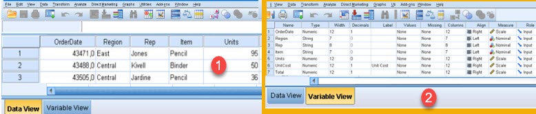
We will see here how to manually enter data into SPSS, or automatically from Excel or from SQL Server. When we open SPSS, we can see Data View (1) and Variable View (2). Data View shows data and is like Excel spreadsheet table. Variable view is used to declare that "Data View" table. There we can declare columns, their content, formatting and possible values.
Manual entry
To enter data manually, it is enough to start typing in the cells in Data View. As we see, names of columns will be created automatically and we have to change them, together with other columns attributes.
Before explaining columns attributes let's recall of different measurement scales that are used in SPSS:
– Nominal scale is used for categorical data ( "man/woman/child" or "India/Japan/China" ).
– Ordinal scale is used for ordered data ( "good/neutral/bad" or "before/during/after" ).
– "Scale" is used in SPSS to label data that can be measured with some measuring unit ( height, weight, temperature ).
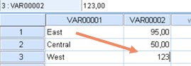
Data that is measured in Nominal and Ordinal scale has to be enter in SPSS as codes. This is is necessary so we can use all available statistical tools in SPSS. Coded means that each category has to be presented by number. For example "small, medium, big" can be presented with codes "1,2,3". Those codes are values that we enter into the program (1). Then, in the program itself, we assign one of the categories labels to each code. If we want, we can show those categories labels to user instead of codes (2).
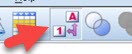
By clicking on this button in the main toolbar, user can switch between the two views from the image above.
Declaration of code is done in "Variable View". Let's see what options are available in Variable View.
Variable View
"Variable View" is place where we enter columns attributes.
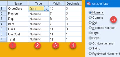
– In "Name" (1) we type correct name of a column. Name can have characters, numbers and underscores.
– In "Type" (2) we open new dialog (5) to choose between different data types. As we saw, because all categorical data should be coded, almost all of our columns should be declared as "Numeric".
– Width (3) is to limit how many characters can textual data has. Textual data longer than this will be truncated.
– Decimals (4) will limit number of decimal places presented in "Data View". This is just for visual representation. Real calculations will be conducted with all available decimal figures.
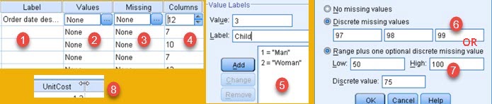
– In "Label" (1) we place short descriptions of our columns.
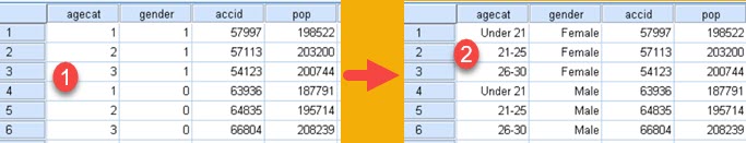
– In "Values" (2) we can set labels for data that is categorical in nature. This will open new dialog (5). So, if possible codes in column are "1, 2, 3" then we have to attribute label to each code. Our codes "1,2,3" can represent "Man, Woman ,Child". By clicking on button in toolbar, as explained earlier, user will be able to see those labels instead of incomprehensible codes.
– In "Missing" (3) we can determine values that are impossible or unacceptable. After we enter data, every value that is the same as those registered here, will be excluded from calculations as incorrect value. Such values will not be part of statistical calculations, SPSS will just ignore them. We can give three such discrete values (6). Other option is to give one interval and one discrete value (7).
– "Columns" (4) is visual width of column, measured in numbers of characters. We can also change width of columns with mouse on the same way as in Excel (8).
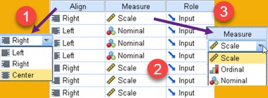
Last 3 column attributes are Align, Measure and Role. In align we can choose between Left, Right and Center alignment (1). Measure (2) is used to declare scale for data. This will not influence SPSS calculations but it is important to declare scale of data for other users of that data. In Role (3) we can just leave the default value ( "Input" ).
This process of declaring our columns should be done for data loaded from Excel or database, too.
Loading from Excel
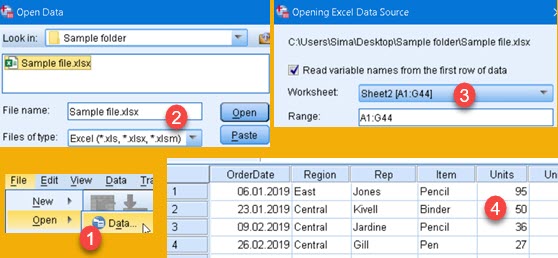
File > Open > Data (1) in the main menu is option to open dialog (2). Dialog (2) needs from us to choose Excel type of files, folder where Excel file is, and concrete Excel file. After clicking "Open" in dialog (2) we will got dialog (3). There we choose one of the Sheets in the workbook and range of our data. If we don't supply range, automatically determined range will be used ( "A1:G44" on image ). After this our data will be loaded and we can see it in "Data View" (4).
Loading from Database
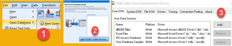
For getting data out of database, "IBM Data Access Pack" can be installed. This is IBM collection of drivers for different databases we can use. We don't have to use IBM drivers, but they will probably work the best, if we want to transfer data to SPSS. We start loading process by clicking on File > Open Database > New Query (1). Then we click button "Add ODBC Data Source" (2). In new dialog, in "User DSN" tab we should click on "Add" button (3).
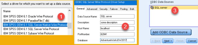
"IBM Data Access Pack" will add many ODBC drivers whose names start with "IBM SPSS OEM" (1). We will choose "SQL Server Native Wire Protocol". In next screen we'll add credentials for our database (2). Now, we will close everything until we get back to our start screen (3), so we can click "Next" button.
Now we can select some table and its columns (1 => 2) and click on Finish. Those columns will be now presented into Data View (3).
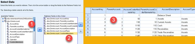
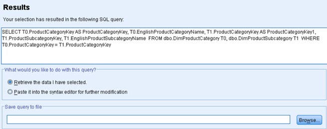
Instead of Finish we can also use Next buttons to follow whole graphical wizard. This wizard will provide us with opportunity to define relations between tables, to filter data and to rename columns. This is all great, but the last screen is where we will be able to see and directly change SQL statement. I find it easiest to make changes here. After this step we have to click on Finish button, wizard will exit, and we will see our data loaded into SPSS program.