Excel

Embedded Custom Icons in Excel File

Sometimes, when we download an Excel file from the Internet, we get icons that are actually previews of the contents of the Excel file. We can get icons like this if we enable thumbnails for Office files. We will see below how to achieve this.

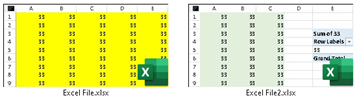
But even better, we can replace those preview icons with our brand icons. So, we get something like the icons below for our Excel files, but also for our Word and PowerPoint files. When we send such files to someone else, that person will receive files with our custom icons. We cannot remove the small images in the corner (1), they are automatically placed by Office, but the rest of the icon is free to customize.

How to Enable Thumbnails for Office Files

When we save files from Excel, Word or PowerPoint for the first time, there is a check box that will produce the saved files with a preview icon. We just need to check that checkbox before saving our file. Programs will remember our setting so the next time we save some other file, this checkbox will be checked. We have to do this separately for Excel, Word and PowerPoint.

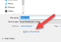
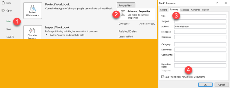
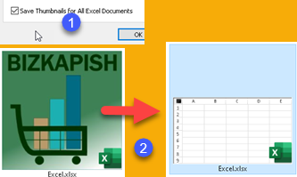
It is also possible to enable this checkbox if we go to File > Info (1) > Properties > Advanced Properties (2). In the new dialog, we would have to go to the Summary tab (3) and there we have to check (4) "Save thumbnails for all Excel documents". "Save Thumbnail" and "Save Thumbnail for All Excel Documents" are the same checkbox and they are always synchronized.

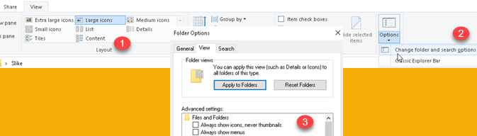
Such preview icons will only be visible on the desktop or within a Windows Explorer window. Within the Windows Explorer window, the View selected should be "Large Icons" or some similar option (1). If we still can't see our preview icon, we should also check inside View > Options > Change folder and search options (2). That will open a new window, where in the View tab we have the option "Always show icons, never thumbnails" (3). We should make sure to disable that option.

Insert a New Icon Manually from Scratch

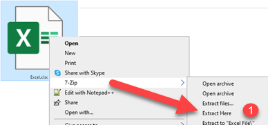
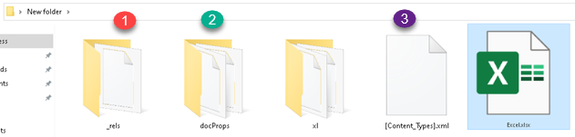
The file formats XLSX, DOCX, PPTX are actually ZIP files. We can use some program that can extract such archives to get the inside of our Office files. In Figure (1) we can see how to use the popular 7-Zip program to extract our archive. For some other programs, you will first need to change the Excel file extension from XLSX to ZIP, and then use that other program to decompress. 7-Zip doesn't need that step, it will happily extract the XLSX file directly.

As we can see below, we would get at least three folders and one XML file from one Excel file. There may be some other files inside, but for our project we are only interested in the folders (1), (2) and the XML file (3).

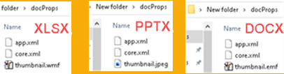
Inside the "docProps" folder we will place our icon. The icon must be in WMF file format for Excel, JPEG file format for PowerPoint, EMF file format for Word. I use a size of 64×64 pixels. The icon names should be "thumbnail.vmf", "thumbnail.jpeg", "thumbnail.emf".

In XML file "[Content_Types].xml", before </Types>, we need to add red text from bellow. For PPTX files, text is almost the same, we just use jpeg format so the text should be "<Default Extension="jpeg" ContentType="image/jpeg"/>". For DOCX files we use "<Default Extension="emf" ContentType="image/x-emf"/>".

…heetml.styles+xml"/><Override PartName="/docProps/core.xml" ContentType="application/vnd.openxmlformats-package.core-properties+xml"/><Override PartName="/docProps/app.xml" ContentType="application/vnd.openxmlformats-officedocument.extended-properties+xml"/><Default Extension="wmf" ContentType="image/x-wmf"/></Types>

Inside the "_rels" folder there is ".rels" XML file. Inside it we do something similar. Before </Relationships>, we need to add red text from bellow.

…nxmlformats.org/officeDocument/2006/relationships/officeDocument" Target="xl/workbook.xml"/><Relationship Id="rId999" Type="http://schemas.openxmlformats.org/package/2006/relationships/metadata/thumbnail" Target="docProps/thumbnail.wmf"/></Relationships>

For Powerpoint files, the only difference for ".rels" file is that we use "thumbnail.jpeg" instead of wmf.

<Relationship Id="rId999" Type="http://schemas.openxmlformats.org/package/2006/relationships/metadata/thumbnail" Target="docProps/thumbnail.jpeg"/>

For word we use EMF.

<Relationship Id="rId999" Type="http://schemas.openxmlformats.org/package/2006/relationships/metadata/thumbnail" Target="docProps/thumbnail.emf"/>

The final step is to zip all the insides of our Excel file back into the ZIP file (1). After that we just change the extension of that ZIP file to XLSX and our custom icon is applied (2).

What if We Already Have a File with a Thumbnail?

In that case, the procedure above is almost the same, but the only modification would be to replace existing WMF (or JPEG or EMF) image with our own. If the office file already has a thumbnail, then there is no need to modify XML files, we just replace the image.

Such Custom Icons are Fragile

If the user opens our file, changes some content, and then he clicks "Save", our custom icon will be lost. There are two scenarios here:

1. If the user has "Save Thumbnails for All Excel Documents" option turned on (1), then our custom icon will change to a preview thumbnail (2).

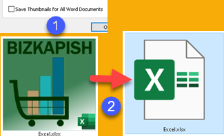
2. If "Save Thumbnails for All Excel Documents" option is turned off (1), clicking on "Save" will revert our custom icon to the standard Excel icon (2).

Changing Default Template

Is it possible to change our default template so that every new Excel file has our custom icon?

Well, that is not possible. You can create a new file from a template, but when you save that file, your custom icon will be removed, so it is not possible to inherit custom icon from the default templates.

How to Automatically Change Office File Icons to Custom Icons

If you have a lot of Office files and want to change their icons to custom icons, then you can use my VBA project which is available for download at the bottom of this blog post. This project will work both on files without preview icon, and on files that have a preview icon. The VBA project will work on all files that have four-character extensions where the first three characters are XLS*, PPT* or DOC*. This means that this VBA project will also change the icons of XLSM and similar files, too.

First download "Icons Customization" folder (1). You can place this folder anywhere and you can rename it. Inside it there is a subfolder "Icons1" (2). Within that subfolder you can find WMF, EMF and JPEG files (3). I also uploaded original SVG files there. I transformed those SVG files into PNG files, and then those PNG files into WMF and EMF files. I couldn't get the correct WMF and EMF files directly from SVG files. The "Icons2" folder is the same as folder "Icons1". You can have up to 20 such folders with different icons sets. These "Icons" subfolders shouldn't be renamed.

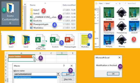
Files "Excel, Powerpoint, Word" (4) are the files that will get a new icon. You can place more Office files here and all of them will be modified. Note that files for Excel and Powerpoint  (5) are regular files, but the Word file (6) has a preview icon.

Now, open the "CHANGE ICONS" file (7). Choose from drop down menu (8) which icon set you want to use. Then run the "subCustomizeIcons" macro (9). When the project is completed, you will get a message (10). If you have many files and if they are big in size, then this procedure will take longer. Every file must be zipped and unzipped, and this takes time.

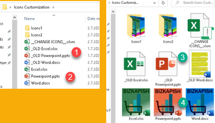
All original files will now be prefixed with "_OLD" (1). The new files will have original names (2). If we switch to "Large icons" view, we will see that our original files are unchanged (3), but our new files have branded icons (4).

From here you can dowload VBA project:

Analysis ToolPak is an Excel add-in that provides many statistical tools. This add-in comes in two flavors, and each of them has to be enabled in "Add-ins" dialog (1) in order to use it. They both have the same functionality but "Analysis ToolPak" has its functionality available only through graphical interface. "Analysis ToolPak – VBA" is accessible both through graphical interface and VBA code.

After we enable "Analysis ToolPak" (1), a button will appear in Data > Analysis (2). By clicking on that button, we will open dialog with many statistical tools (3). In order to use any of these tools we just have to select it and click on OK. New dialog will appear which provides options for that specific statistical tool.

Descriptive Statistics

Descriptive statistics is based on a brief descriptive coefficients that quantitatively describe or summarize features of a data set. Data set is set of results of measurements made on a population or a sample. This coefficients comprise measures of central tendency like mean, median, mode, and measures of variability like Standard error, Variance, Range, Kurtosis.

We will select "Descriptive statistics" tool in Analysis ToolPak. "Descriptive statistics" dialog asks us to enter what range will be used as a source of data (1). This range, in our example, has two columns and we will get results for each of them. Program doesn't know whether data in selected range is organized in Columns or Rows. We will choose Columns (2) in our case, to solve that dilemma. Our data has labels in the first row, so we have to check option (3) in order to have first row excluded from calculations.

Final output can be directed to a range in the same sheet or some other sheet in the same workbook (A). This range is defined by it's top left cell. Option (B) means that new sheet will be created with provided name and result will be pasted in "A1" cell in that new sheet. Selection of option (C) will create new workbook with the name "Book1", and the result will be pasted in sheet "Sheet1" in cell "A1" in that workbook.

Last options (4,5,6,7) are for selecting what results should be calculated. Option (4) "Summary statistics" should always be selected because without it most of important indicators (mean, variance…) will not be part of a final result. Option (5) needs confidence level for calculating confidence interval for the mean. Without it checked, we will not get this result. Options (6,7) will give us the same results as SMALL and LARGE functions in Excel.

Descriptive Statistics Results

This is what the results of descriptive statistics would look like. We have results both for Col1 and Col2. For each column there is a list of different indicators which describe our data set. We will only analyze results for the first column.

To the right, we can see all the results for first column, with the same results calculated by using Excel formulas. We can see that all the results are the same but there is one potential difference. If there are multiple values in data set that could be considered as Mode ( e.g. 1,1,2,5,5 ), Analysis ToolPak would return the last one ( 5,5 ), but the MODE function would return the first one ( 1,1 ).

Formulas used in Analysis ToolPak descriptive statistics

Bellow are listed formulas used for calculation of some descriptive indicators.

Standard Deviation		Variance
Standard Error		Confidence Interval
Kurtosis		Skewness

Let's calculate Confidence Interval by using its formula. Because our sample is smaller than 30 observations, we will use t distribution. For 95% confidence level, with 3 degrees of freedom, t value would be 3.1824. That means that t * s_x̄ = 3.1824 * 0,75 = 2.3868. This is the same result as Excel CONFIDENCE.T function is returning. Now our confidence interval is ( 2,75 – 2,3868; 2,75 + 2,3868 ), which is ( 0,3632; 5,1368 ).

Kurtosis and Skewness are used to describe how much our distribution fits into normal distribution. If Kurtosis and Skewness are zero, or close to zero, then we have normal distribution.

Analysis ToolPak Descriptive Statistics through VBA

Descr Subprocedure

Different functionalities of Analysis ToolPak can be called through VBA subprocedures. Bellow we can see how to provide arguments and call procedure with the name "Descr" for descriptive statistics. All arguments except the first one are optional. All arguments are of a type Variant.

Sub subDescrFunction()
Dim inputRng As Range: Set inputRng = Range("Sheet1!A3:B7")
Dim outputRng As Range: Set outputRng = Range("Sheet1!K3")
Application.Run "Descr", inputRng, outputRng, "C", True, True, 1, 1, 95
End Sub

inprng	This is input range, with our data set.
outrng	This is output range. Output range is declared with a reference to a top left cell of the output range. If we type some word here, Analysis Toolpak will export result into new worksheet with such name. If this argument is False, blank or omitted, new workbook will be created.
grouped	Is our data set organized in rows or columns? Depending on that, we type "R" or "C". "C" is default.
labels	Here we should type "True" if our data set has header. If False or omitted, then we claim that there are no labels.
summary	Type "True" to get all major descriptive statistics. If this argument is False, blank or omitted, those values will not be calculated.
ds_large	What k-th largest value to get? If this argument is omitted, this value will not be calculated.
ds_small	What k-th smallest value to get? If this argument is omitted, this value will not be calculated.
confid	What is confidence level for calculating confidence interval for the mean? If this argument is omitted, there will be no result.

VBA project for Analysis ToolPak (ATPVBAEN.XLAM) is protected with the password "Wildebeest!!". There you can find declarations of all VBA procedures.

DescrQ Subprocedure

There are two variants of subprocedures for descriptive statistics. First has name Descr, and the second one has name DescrQ. "Descr" would create result immediately by using arguments provided in the code. "DescrQ" would first open GUI dialog filled with values provided in the code (1). We can then accept those values, or we can change them, and then we can click on OK button. Only then, final results will be created (2). "DescrQ" give us opportunity to customize values provided in the code.

All the code for "Descr" and "DescrQ" is the same. Only difference is the name of subprocedure.

Application.Run "DescrQ", inputRng, outputRng, "C", False, True, 1, 1, 95

"DescrQ" version has one bug. Ranges in the dialog will have starting "grave accent" missing. [New Microsoft Excel Worksheet.xlsm]Sheet1'!$D$9:$D$12 'initial formatting '[New Microsoft Excel Worksheet.xlsm]Sheet1'!$D$9:$D$12 'corrected starting sign

Sample file can be downloaded here:

Today() function is one of volatile functions in Excel. Volatile functions are recalculated each time any cell in the spreadsheet is changed. Some other actions can also cause recalculation, such as renaming sheets, inserting columns, deleting rows, etc. If you have many cells in Spreadsheet that are referring to cell that contains Today() function or you have many cells using Today() function, everything in your file will slow down. Constant recalculations will make working in such file really unpleasant experience.

Today() function will change its result only when the new day arrives. Because of this we can find another way to get today's date. There are actually several ways to accomplish this.

Offline Solutions

VBA Solution

In VBA, if we place "Application.Volatile" as the first line in our UDF (User Define Function), that function will become volatile. We will not do that. That way we can make VBA UDF function that is not volatile and it is replacement for Excel today() function. This function will refresh itself each time we open the file.

Function vbaToday() As Date vbaToday = Date End Function

User now just have to type "=vbaToday()" into spreadsheet and he will get today's date inside that cell.

Power Query Solution

We will first make a query that only returns today's date.

let Source = #table( type table [ #"pqToday"=date ] , { { DateTime.Date(DateTime.LocalNow()) } } ) in Source

We will load this query into spreadsheet so that we have today's date in cell A3.

We will then set the option so that query is refreshed every time the file is opened.

In the pane with the queries (1), we should right click on our query and choose its Properties (2). In the new dialog we want to check option "Refresh data when opening the file" (3).

Possibility of error

There is a small problem with VBA and Power Query solutions. If we open the file just before a midnight, when the midnight pass, new day will arrive, but our date will not change. For VBA solution, we would need to enter the cell with F2 and press Enter ( F9 and Calculate Now would not work on UDF function ). For Power Query solution we would need to Refresh our query.

Closing and opening the file would also give us new date, or we can just turn off our computer and go to sleep before midnight.

Online Solution

Power Automate Solution

VBA and Power Query will not work for Excel online. We can use Power Automate to change date in one cell every day in midnight. We will combine Power Query solution and Power Automate solution, so that it doesn't matter if file is in cloud or on user's computer. First, we will change our query because Power Automate needs one more column. We are going to add "Key" column to our Power Query table.

let Source = #table( type table [ #"Key"=text, #"pqToday"=date ] , { { "paDate", DateTime.Date(DateTime.LocalNow()) } } ) in Source

Now we can create flow that will change date in cell B3 every day in midnight.

We click on "Create" button (1) for the new flow. Then we select "Scheduled cloud flow" (2). We will be offered dialog where we give our flow name (3), we can decide that from now, each day the flow will run (4,5). Next, we will get diagram view with "Recurrence" as the first step (6). As a next step we will add "Update a row" (7). Now that we have both our steps (8), we can fill necessary data. In Recurrence step we just have to show advanced options (9) and decide what time zone should be used (10). In "Update a row" step we have to write where is our file and what is its name (11,12). (13) is the name of the declared table in which we are going to insert today's date. "Key" column is considered as primary key column so we have to give a value for primary key which defines row where we want changes to happen (14). Name of declared table is "pqToday". That row is made of fields. Those fields will appear at the bottom (15). We have only one field to fill. In this field we will write: convertFromUtc(utcNow(),'Central Europe Standard Time','dd.MM.yyyy'). This code will take current date according to given time zone and it will format it. This date will be written to our Excel file in cell B3. For some reason step "Update a row" wasn't able to find my Excel file when I was using XLSM extension. It seams that file has to be XLSX.

Sample file can be downloaded from here:

We have our PBIX file opened (1). Our Excel is also opened. We click on button in the ribbon (2) and new pivot table is added to active sheet (4). This pivot table is connected to our PBIX file. Now we can easily create pivot table by using data from Power BI Desktop.

After closing Power BI Desktop, our pivot table will be non interactive. We can open PBIX file again, but this time Power BI Desktop will have some other credentials. This mean that our pivot table will still be non interactive. We have to click on button (3) "Reconnect" to establish connection again. Now we can use our pivot again.

This post will not explain how to create buttons (2,3). It will only explain VBA code needed to achieve described functionality. Code is simple, so it will work with only one PBIX file. Name of that file is hardcoded. This code has no error handling.

Structure of code

On the top we have two procedures "subCreateNewPivot" (1) and "subReconnect" (2). Beside them we have two groups of functions. "Red Orange" group is used to provide credentials of our PBIX file. "Green" group is used to create pivot table. "subCreateNewPivot" is using both groups, but "subReconnect" is using only the "red orange" one.

As explained in one of previous posts, each time Power BI Desktop is opened, it has different credentials and it writes them into location:
C:\Users\<Username>\AppData\Local\Microsoft\Power BI Desktop\AnalysisServicesWorkspaces (1)
That location has several subfolders (2), each for any of opened Power BI Desktop files. Sometimes there are subfolders that belong to already closed PBIX files, but this subfolders are incomplete and they will be deleted automatically after some time. Inside those subfolders there are two important files. File (3) has name of database in its name ( 601ae6aa-a3c6-4abb-8833-2253863854e4 ). File (4) is ordinary TXT file and it has port number of Power BI Desktop server as its only content.

There are two problems with this setup:
1) Credentials are changed each time Power BI Desktop is opened.
2) We don't know which credentials belong to which opened PBIX file.

Solution is to read all available credentials with function "funcAllCredentials". This function is using two helper functions "funcPort" and "funcDatabaseName". Those helper functions reads values of port number and database name from computer disk. This credentials are then given to function "funcPowerBIpivotDataCredentials" which have to decide which of credentials are the ones we are looking for. We are looking for credentials of "PowerBIpivotData" file. In order to identify correct credentials we are going to read values from tables that we previously created in all of our Power BI Desktop files. Each our PBIX files has table named "NameValue" that looks like (1,2). We will use function "funcPBIXname" to read from each open PBIX file from such table. If, by using some of credentials, we read the value "PowerBIpivotData" (1) from some of the opened PBIX files, that would indicate that those are credentials we need.

Credentials are all we need for "Reconnect" functionality. Procedure "subReconnect" will look for connection that has name starting with "PowerBIpivotData". This indicate connection that was created before, to create pivot tables. Procedure will then update this connection and its name with new credentials. After this, pivot tables will become interactive again.

Pivot table creation

"New pivot" button also needs information about credentials. This button will use those credentials to create new pivot table. Top procedure "SubCreateNewPivot" will call procedure "subNewPivot", and that procedure will create new pivot table, by using provided credentials. First, procedure subNewPivot will chech whether connection already exists. If we previously created some pivot table, then we already have connection and we don't have to create new one. We are using helper function "funcConnectionMissing" to check existance of such connection. If this is not true, then we will create new connection.

New connection will be used to create new pivot table. New pivot table will be created in the top left cell of user selection in the spreadsheet.

VBA code

VBA code is long enough to not be shown in the text of this blog. Bellow is link for downloading Excel file that has all VBA code and buttons in its ribbon tab. PBIX files are also included.

While typing some formula, we can click on spreadsheet cell to get its reference. If the cell is inside declared table, our reference will be structured reference.

Structured reference works by cutting horizontal and vertical slices of a table, and then it returns intersection of those slices.

Vertical slicing can be done in two ways. We can slice only one column, and we can slice several consecutive columns.

Combining specifiers

Now we have to use two specifiers. First we write horizontal specifier, and then the vertical one. Yellow example bellow, returns whole "Units" column because horizontal specifier is [#All]. Blue example returns headers for two consecutive columns because horizontal specifier is [#Headers]. Red example is different. It uses two horizontal specifiers. This way we can only use combinations ( [#Data],[#Headers] ) and ( [#Data],[#Totals] ). Red example returns "Total" column without its header. Green example assumes that formula is in the sixth row. That is why it returns values for columns "Region" and "Rep" in sixth row.

It is not possible to combine [#All] specifier, or [@] specifier with some other. They only goes alone.
Specifier for "current row" is not separated with coma, there is no coma between "@" and name of column. If we want current value for only one column we type "=SampleTable[@ColumnName]".

Choose function

Choose function can help us to solve two problems. First is, that we want to reference several not consecutive columns from the table. Let's say that we want to reference columns "Region" and "Total", but we don't want their [#Totals]. We can use this formula:

=CHOOSE({1,2},SampleTable[[#Headers],[#Data],[Region]], SampleTable[[#Headers],[#Data],[Total]] )

If we want to wrap two columns into one aggregate function, we don't need Choose function, we can directly type columns references as arguments into function. Function bellow will return 2339,36 ( 264 + 2075,36 ).

=SUM(SampleTable[Units],SampleTable[Total])

Other problem is that we can not combine [#Headers] and [#Totals]. Solution is again to use Choose function. Notice that this time "{1;2}" argument is using semicolon, and not coma.

=CHOOSE({1;2},SampleTable[#Headers],SampleTable[#Totals])

Relativity of structured references

If we copy formula with structured reference to some other cell (1), it will not adapt. We can see in cells A10:D10, in image bellow, that all cells have the same value. Sometimes this behavior is desired, but sometimes is not.

Things to consider about structured references

Structured references are easy to read, but not to type. Usually we just click on some table cell and Excel creates structured reference for us. If this is not what we want, it is possible to disable automatic creation of structured references. This is done by unchecking option in Excel Options > Formulas > Working with formulas > Use table names in formulas. VBA version of this would be:

Application.GenerateTableRefs = xlGenerateTableRefA1   'to turn automatic creation OFF
Application.GenerateTableRefs = xlGenerateTableRefStruct  'to turn automatic creation ON

Structured references can be used inside VBA. Here is one example:

Worksheets(1).Range("Table1[#All]")

Declared table doesn't need to have headers and total row. They can be disabled in Table Design > Table Style Options, in Excel ribbon. After this, formulas which refer to [#Headers] or [#Totals] will not work.

Column names can be qualified and unqualified. Unqualified names can only be used inside tables. This means that instead of writing SampleTable[Region] we can just type [Region]. This will not work outside of table which has "Region" column.

In ribbon, there is option to convert declared table into ordinary range. That option is in Table Design > Tools > Convert to range. After this, all structured references for that table will be transformed into regular A1 references.

For special signs [ ] # ' we have to include escape sign – single quotation mark (').

=DeptSalesFYSummary['#OfItems]

File with examples can be downloaded here: