Descriptive statistics
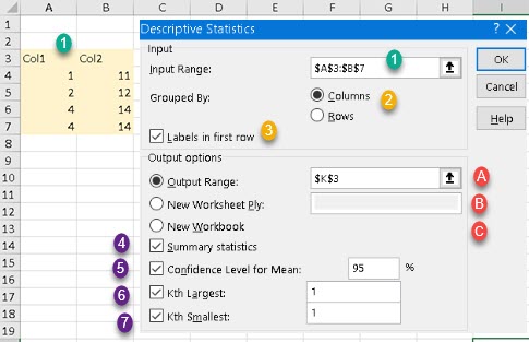
Descriptive statistics is a branch of statistics that is describing the characteristics of a sample or population. Descriptive statistics is based on brief informational coefficients that summarize a given data set. In descriptive statistics we are mostly interested in next characteristics:
- Frequency Distribution or Dispersion, refers to the frequency of each value.
- Measures of Central Tendency, they represent mean values.
- Measures of Variability, they show how spread out the values are.
Frequency Distribution
Frequency distribution shows how many observations belong to different outcomes in a data set. Each outcome can be described by group name for nominal data or ordinal data, interval for ordinal data or range for quantitative data. Each outcome is mutually exclusive class. We just count how many statistical units belong to each class.
Frequency distribution is usually presented in a table or a chart. There are four kinds of dispersion tables. For each kind of table there is a convenient chart presentation:
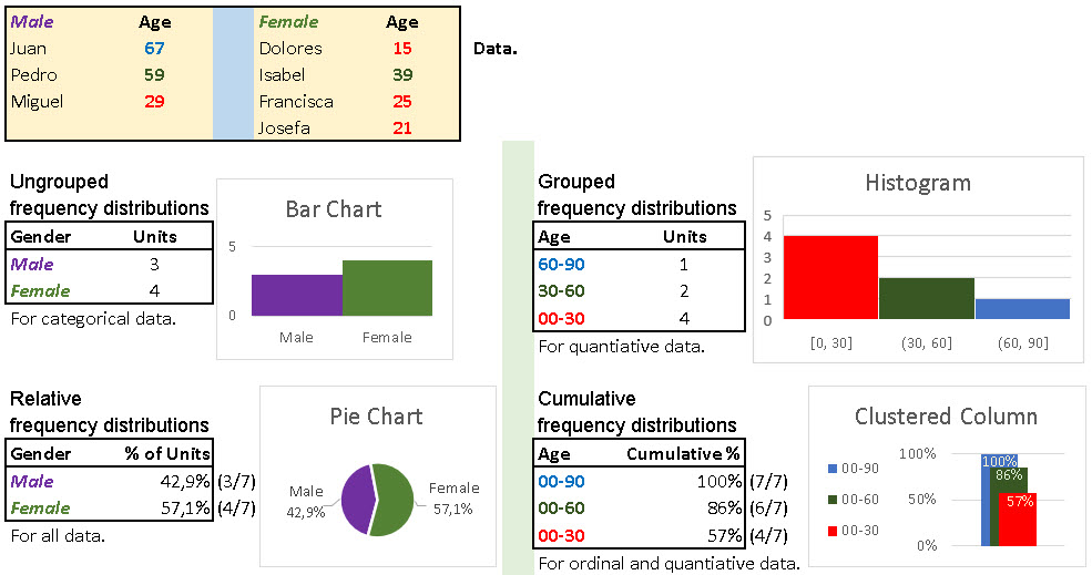
– Ungrouped frequency distributions tables show number of units per category. Their counterpart is Bar Chart.
– Grouped frequency distributions tables present number of units per range. Their companion is Histogram.
– Relative frequency distributions tables show relative structure. Their supplement is Pie Chart.
– Cumulative frequency distributions tables are presenting accumulation levels. Their double is Clustered Column chart.
Measures of Central Tendency
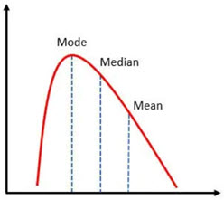
Measures of central tendency represent data set as a value that is in the center of all other values. This central value represents the value that is the most similar to all other values and is the best suited to describe all other values through one number. There are three measures of central tendency, Average, Median and Mode. In normal distribution these three values would be the same. If we don't have symmetry, then Median would be closer to extreme values then the Average, and Mode be at the top of distribution.
Average
Average is calculated by summing all the values, and then dividing the result with number of values ( x̄ = Σ xi / n ).
Median
The median is calculated by sorting a set of data and then picking the value that is in the center of that array. Let's say that all values in array are indexed from 1 to n [ x(1), x(2)…x(n-1), x(n) ].
If number of values in array is odd, median is decided by index (n+1)/2. Median is then decided like x̃ = x(n+1)/2, like in array [ 9(1), 8(2), 7(3), 3(7+1)/2, 1(5), -5(6), -12(7) ]. There are an equal number of values before and after median in our array, 3 values before the median and three values after the median.
If number of values is even, formula is x̃ = (x(n/2)+x(n/2)+1)/2, like in [ -3(1), 1(2), 0(3), 2(8/2), 3(8/2)+1, 4(6), 6(7), 9(8) ], so we calculate an average of two middle numbers (2+3)/2 = 2.5. Again, there are an equal number of values in our array before and after the two central values. As we can see, it is not important whether numbers are arranged in ascending or descending order.
Mode
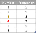
The mode is the most frequent value in a sample or population. One data set can have multiple modes. In sample ( 1, 3, 2, 3, 3, 5, 4, 4, 8, 4 ) we have two modes. Both the numbers 3 and 4 appear three times. If we create Ungrouped Frequency Distribution table, we can easily notice our modes.
Measures of Variability
Measures of Variability shows how spread out the statistical units are. Those measures can give us a sense of how different the individual values are from each other and from their mean. Measures of Variability are Range, Percentile, Quartile Deviation, Mean Absolute Deviation, Standard Deviation, Variance, Coefficient of Variation, Skewness and Kurtosis.
Range
Range is a difference between maximal and minimal value. If we have a sample 2, 3, 7, 8, 11, 13, where maximal and minimal values are 13 and 2, then the range is: range = xmax – xmin = 13 – 2 = 11.
Percentile
Let's say that we have sample with 100 values ordered in ascending order ( x(1), x(2)…x(99), x(100) ). If some number Z is bigger than M% values from that sample, than we can say that Z is "M percentile". For example, Z could be larger than 32% of values ( x(1), x(2)… x(32), x(33), x(99), x(100) ). In this case x(33) is "32 percentile".
For this sample [ -12(1), -5(2), 1(3), 3(4), 7(5), 8(6), 9(7) ], number 7 is larger than 4 values, so seven is "57 percentile". This is because 4 of 7 numbers are smaller than 7, and 4/7 = 0,57 = 57%. Percentile show us how big part of sample is smaller than some value.
Be aware that there are several algorithms how to calculate percentiles, but they all follow similar logic.
Percentiles "25 percentile", "50 percentile", "75 percentile" are the most used percentiles and they have special names. They are respectively called "first quartile", "second quartile" and "third quartile", and they are labeled with Q1, Q2, Q3. Quartile Q2 is the same as median.
Quartiles, together with maximal and minimal values divide our data set in 4 quarters.
xmin [25% of values] Q1 [25% of values] Q2 [25% of values] Q3 [25% of values] xmax
Quartile Deviation
The difference of third and first quartile is called "interquartile range": QR = Q3 – Q1. When we divide interquartile range with two, we get quartile deviation. Quartile deviation is an average distance of Q3 and Q1 from the Median.
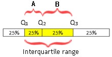 | Average of ranges A and B is quartile deviation, calculated as: QD = (Q3 – Q1 ) / 2. |
Mean Absolute Deviation
Mean absolute deviation (MAD) is an average absolute distance between each data value and the sample mean. Some distances are negative and some are positive. Their sum is always zero. This is a direct consequence of how we calculate the sample mean.
| x̄ = Σ xi / n n * x̄ = Σ xi n * x̄ – ( n * x̄ ) = Σ xi – Σ x̄ 0 = Σ ( xi – x̄ ) | We can see, on the left, that formula, used for calculation of a mean, can be transformed to show that sum of all distances between values and the mean is equal to zero. This is why, for calculating mean absolute deviation (MAD) we are using absolute values. | 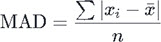 |
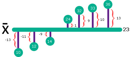 | If our sample is [ 10, 12, 14, 24, 32, 33, 36 ], mean value is 23. Sum of all distances is ( -13 – 11 – 9 + 1 + 9 + 10 +13 ) = 0. Instead of original deviations we are now going to use their absolute values. So, sum of all absolute deviations is ( 13 + 11 + 9 + 1 + 9 + 10 + 13 ) = 66. This means that MAD = 66 / 7 = 9,43. |
Standard Deviation and Variance
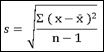
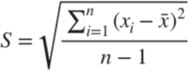
The standard deviation is similar to the mean absolute deviation. SD also calculates the average of the distance between the point values and the sample mean, but uses a different calculation. To eliminate negative distances, SD uses the square of each distance. To compensate for this increase in deviation, the calculation will ultimately take the square root of the average squared distance. This is the formula used for calculating standard deviation of the sample:
 | Variance is just standard variation without root => |
Standard deviation is always same or bigger than mean absolute deviation. If we add some extreme values to our sample, then standard deviation will rise much more than mean absolute deviation.
Coefficient of Variation
Coefficient of variation is relative standard deviation. It is a ratio between standard deviation and the mean. The formula is CV = s / x̄. This is basically standard deviation measured in units of the mean. Because it is relative measure, it can be expressed in percentages.
Let's imagine that the standard deviation of a giraffe's height is equal to 200 cm. Standard deviation of a mouse's height could be 5 cm. Does that mean that variability of giraffe's height is much bigger than variability of mouse's height? Of course it is not. We have to take into account that giraffes are much bigger animals than mice. That is why we use coefficient of variation.
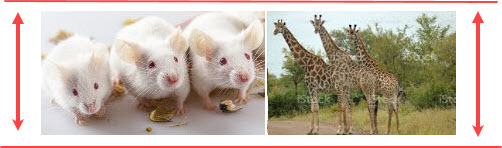 | If we scale the images of mice and giraffes to the same height, we can see that the relative standard deviation of their heights is not as different as the ordinary standard deviation would indicate. |
Kurtosis and Skewness
Kurtosis and Skewness are used to describe how much our distribution fits into normal distribution. If Kurtosis and Skewness are zero, or close to zero, then we have normal distribution.
Skewness is a measure of the asymmetry of a distribution. Sometimes, the normal distribution tends to tilt more on one side. If skewness is positive then distribution is tilted to right side, and if it is negative it is tilted to left side.
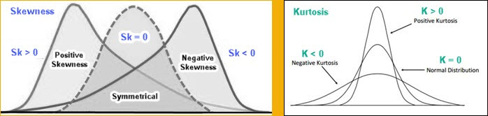
If skewness is absolutely higher than 1, then we have high asymmetry. If it is between -0,5 and 0,5, then we have fairly symmetrical distribution. All other values mean that it is moderately skewed.
| To the right we can see how to calculate Skewness statistics. |  |
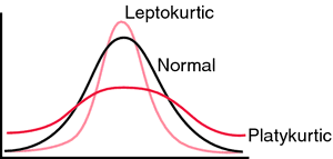
The Kurtosis computes the flatness of our curve. Distribution is flat when data is equally distributed. If data is grouped around one value, then our distribution has a peak. Such humped distributions mean that kurtosis statistics is positive. That is Leptokurtic distribution. Negative values of kurtosis would mean that distribution is Platykurtic. The distribution is then more flat. Critical values for kurtosis statistics are the same as for skewness.
 | To the right we can see how to calculate Kurtosis statistics. | 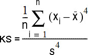 |