OCR a PDF Document With Python and Tesseract
We have a pdf document that is like a picture. We want to turn it into searchable document. We will use python Pytesseract module to do the transformation.
WinPython
For this demonstration I will use WinPython distribution. This distribution has size of 813 MB for download. When decompressed this archive will become a 4 GB folder. Choose wisely where to place this folder because latter moving or deleting this folder could take some time.
I am using WinPython distribution because it has many modules already preinstalled, and this will save us some effort. It will also keep us from dependency hell problems.
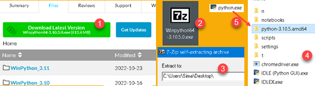
We can download WinPython from this page "https://sourceforge.net/projects/winpython/files/". On that page click on the green button (1) and download EXE file on your computer (2). This file is self-extracting archive (3). Choose where do you want this file to be extracted. You will get a folder (4). In the subfolder "python-3.10.5.amd64" (5), of that folder, there is "python.exe" file.
PATH Environment Variable
Windows has a small key-value "database", where each key-value pair is one environment variable. We can open dialog with those variables by going to Run dialog (shortcut Win+R), and typing "sysdm.cpl" (1). In the new dialog we will go to Advanced tab (2), we will click on "Environment variables" button (3), and then we will see dialog with a list of all the key-values pairs (4,5) for environment variables. Some variables are available only for the logged user (6), and system variables are available for all the users (7).
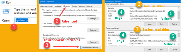
For example, there is key-value pair TEMP = "C: \Windows \TEMP". This allows every program to easily find where Windows temporary folder resides. If Microsoft change the location of this folder, all other programs will still work correctly because they will read that new location from the environment variable. Name of a key is stable, only value is changing, so environment variables are used for communication between programs.
There is an environment variable named PATH. We will change value of this variable so we could easily use our WinPython. In user variables (1) find a variable named "Path" (2). Click on Edit button (3), and then, in a new dialog, click on button "New" (4). This will create a place where we can paste our python folder (5). Python folder is a folder where "python.exe" file resides.
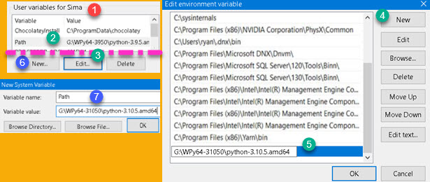
If we don't have Path variable, then we click on "New" button (6) and we fill new dialog with the variable name and variable value (7). Now, python location is added to path variable.
Tesseract
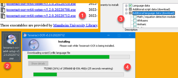
Tesseract is an open-source optical character recognition software. Python is using this software for OCR. First, we go to address https://digi.bib.uni-mannheim.de/tesseract/, and from there we download this software. We will download latest version (1). After EXE file is downloaded to our computer (2), we will start installation. During the installation we can choose (3) additional scripts (Latin, Cyrillic…) and languages (Serbian, Romanian…). Selected scripts and languages will be downloaded during installation (4).
| Folder with "tesseract.exe" file should be added to our path user environment variable ( "C:\Program Files\Tesseract-OCR" ). Now that both python and Tesseract are on the path, we can check whether they are correctly installed. Go to windows command prompt and type commands "python –version" and "tesseract -v". We will now see what versions are installed on our computer. | 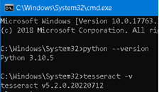 |
There is no need to change working directory inside command prompt. Windows will find both python and Tesseract because they are on the path. This is why we placed them in this environment variable in the first place. Now it is much easier to find these two programs.
Pytesseract
| Pytesseract is python module which communicate with Tesseract software. We will use "pip" module for its installation. Go to command prompt and type command "python -m pip install pytesseract" (1). After successful installation we can check our installed modul with command "python -m pip show pytesseract" (2). | 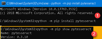 |
Poppler
| Poppler is open-source library for PDF rendering. Go to web site https://blog.alivate.com.au/poppler-windows/ and download latest poppler (1). Downloaded file will be "7z" archive. Extract files from that archive into folder of your choice. Poppler's folder has subfolder "bin" (2). We should add this "bin" folder to path user environment variable. | 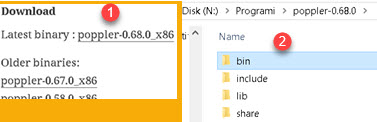 |
Pdf2image
| Pdf2image is python module for interacting with poppler program. We will install it in the same way as pytesseract module. We'll use "python -m pip install pdf2image" (1) and "python -m pip show pdf2image" (2). | 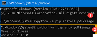 |
Python IDE
We finally have all the ingredients for our project. Now, we will open our favorite python IDE or text editor. If you don't have one, you can go to WinPython folder. Inside it, there is a file "Spyder.exe". Click on this file and you will get Spyder IDE where we can test our code.
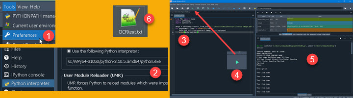
Before running the script, we will first tell Spyder what python.exe to use. Go to Tools > Preferences (1). In the new dialog, type location of our WinPython python.exe file in "Python interpreter > Use the following Python interpreter" (2).
Now we can paste our python script in the pane (3) of the Spyder, and click the Run button (4). OCR-ed text will appear in the console (5) and will also appear as a TXT file on our desktop (6).
Python Script
This is code we are using for our OCR. First, we transform our PDF to sequence of images, using "pdf2image" module. For each page in that sequence, we apply tessarect image_to_string method. This will create our final result. At the end, we write our result in console and in TXT file.
image = pdf2image.convert_from_path('C:\\Users\\Sima\\Desktop\\OCRfile.pdf')
with open('C:\\Users\\Sima\\Desktop\\OCRtext.txt', 'w') as file:
for page number, page in enumerate(image):
detected_text = pytesseract.image_to_string(page)
print( detected_text )
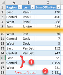
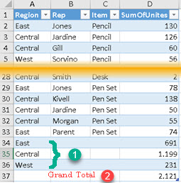
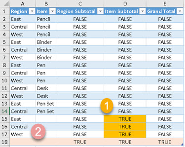
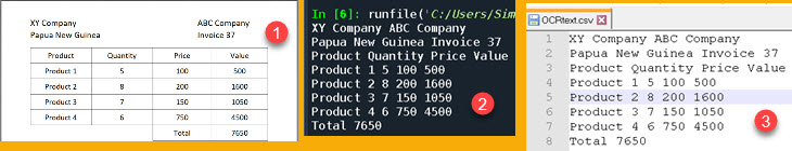
file.write( detected_text )Bellow, we can see how our pdf document looks like as an original (1), in console (2) or in TXT file (3).
Here is the sample file. It contains python script, sample PDF file and poppler software.