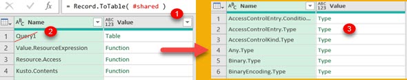
Power Queryhas built-in record with identifier #shared. This record will give us all identifiers that exist in Power Query in current context, and their types. We will transform this record into table and we will then remove this query itself from the list of identifiers, in order to avoid cyclic reference. We will filter only identifiers that represent some of Power Query types. At the end we will sort by type name.
let
IdentifiersAndTypes = Record.ToTable(#shared)
, RemoveItself = Table.SelectRows(IdentifiersAndTypes, each [Name] <> "Query1" )
, FilterOnlyTypes = Table.SelectRows( RemoveItself, each Value.Type( [Value] ) = Type.Type )
, SortTypes = Table.Sort( FilterOnlyTypes, { "Name", Order.Ascending })
in
SortTypes
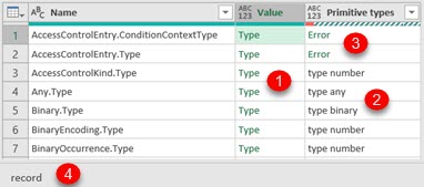
#Shared (1) returned all identifiers in Power Query, together with their types. We will delete (2) the name of our query from this list in order to avoid cyclic reference. We will filter only identifiers that refer to Power Query types (3).
Result will show us, that there are 63. built in types in Power Query. They are presented below.
AccessControlEntry.ConditionContextType
Compression.Type
Guid.Type
MissingField.Type
RelativePosition.Type
AccessControlEntry.Type
CsvStyle.Type
Identity.Type
None.Type
RoundingMode.Type
AccessControlKind.Type
Currency.Type
IdentityProvider.Type
Null.Type
Single.Type
SapHanaDistribution.Type
Date.Type
Int16.Type
Number.Type
Table.Type
SapHanaRangeOperator.Type
DateTime.Type
Int32.Type
ODataOmitValues.Type
Text.Type
SapBusinessWarehouseExecutionMode.Type
DateTimeZone.Type
Int64.Type
Occurrence.Type
TextEncoding.Type
Any.Type
Day.Type
Int8.Type
Order.Type
Time.Type
Binary.Type
Decimal.Type
JoinAlgorithm.Type
Password.Type
TraceLevel.Type
BinaryEncoding.Type
Double.Type
JoinKind.Type
Percentage.Type
Type.Type
BinaryOccurrence.Type
Duration.Type
JoinSide.Type
PercentileMode.Type
Uri.Type
Byte.Type
ExtraValues.Type
LimitClauseKind.Type
Precision.Type
WebMethod.Type
ByteOrder.Type
Function.Type
List.Type
QuoteStyle.Type
Character.Type
GroupKind.Type
Logical.Type
Record.Type
Primitive types
Most of those types above are so called "ascribed types". It means that we can declare them, Power Query will remember them, but it will not enforce them. Power Query only enforce primitive types. This is list of primitive types in Power Query:
type any
type anynonnull
type binary
type date
type datetime
type datetimezone
type duration
type function
type list
type logical
type null
type none
type number
type record
type table
type text
type time
type type
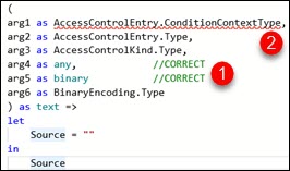
If we try to define a function, arguments can only be declared as primitive types. We can see on the image that only primitive types any, binary, text are colored green by intelisense (1). Even the longer syntax like "Any.Type" is not acceptable. All other types (2) are incorrect and can not be used.
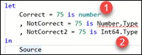
It is the same if we want to use "is" operator. This operator will only work with primitive types ( number is green by intelisense (1) ). Even the longer syntax "Number.Type" will not work. We have to type exactly "number".
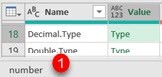
If we select the cell with "Decimal.Type" type in our #shared table, we will see in graphic interface that this type is actually of "number" type (1). It is the same for many other types "Double.Type", "Int16.Type", "Int64.Type", "Percentage.Type" etc., "number" is their real type.
We can create a function that will return primitive type for each of our 63. built in types in Power Query. This is the function:
( TypeToName as type ) as text =>
let
      ListOfTypes = { type any, type anynonnull, type binary, type date, type datetime
        , type datetimezone, type duration, type function, type list, type logical
        , type null, type number, type record, type table, type text, type time, type type }
    , ListOfTypeNames = { "type any", "type anynonnull", "type binary", "type date"
        , "type datetime", "type datetimezone", "type duration", "type function", "type list"
        , "type logical", "type null", "type number", "type record", "type table", "type text"
        , "type time", "type type" }
    , ZipedTypes = List.Zip( { ListOfTypes, ListOfTypeNames } )
    , NameForType = List.Select( ZipedTypes, each  Type.Is( _{0}, TypeToName ) ){0}{1}
in
    NameForType
By using the function above, we will create column "Primitive types". We can see that for each built in type (1), we can get one primitive type (2). This is true for 59/63 built in types. For some built in types (3), we will get Error. In graphic interface we can see that such types are either record or function(4).
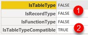
The reason for Error in image above is in the fact that table, function and record types are abstract types. There is no value that has type of table, function of record. We can create one table, record and function and compare their types with such abstract types, but the result will never be TRUE.
let
      Table = #table( { "Column" }, { { "Value" } } )
    , Record = [Field="Value"]
    , Function = () => let Result = "Value" in Result
    , IsTableType = Value.Type( Table ) = type table
    , IsRecordType = Value.Type( Record ) = type record
    , IsFunctionType = Value.Type( Function ) = type function
    , IsTableTypeCompatible = Type.Is( Value.Type( Table ), type table )
in
    [ IsTableType=IsTableType, IsRecordType=IsRecordType
    , IsFunctionType=IsFunctionType, IsTableTypeCompatible=IsTableTypeCompatible ]
We can see that equality will never be reached (1). But if we use "Type.Is" function to check compatibility with primitive types we will get TRUE. Compatibility means that any table is compatible with the "type table". The same is true for records and functions.
When we declare type for function arguments, that argument will accept any value that is compatible with our declaration. If our argument is of type "number", such argument can receive values of all the compatible types "Double.Type", "Int16.Type", "Int64.Type", "Percentage.Type" etc.
How to check ascribed type
We will create three values of type Int64.Type, Decimal.Type andText.Type. The question is how to read ascribed types of this values. We can do that from "metadata".
Value.Metadata function will return record which has Documentation.Name fild which contains ascribed type name. This is where Power Query store information about ascribed types.
Today() function is one of volatile functions in Excel. Volatile functions are recalculated each time any cell in the spreadsheet is changed. Some other actions can also cause recalculation, such as renaming sheets, inserting columns, deleting rows, etc. If you have many cells in Spreadsheet that are referring to cell that contains Today() function or you have many cells using Today() function, everything in your file will slow down. Constant recalculations will make working in such file really unpleasant experience.
Today() function will change its result only when the new day arrives. Because of this we can find another way to get today's date. There are actually several ways to accomplish this.
Offline Solutions
VBA Solution
In VBA, if we place "Application.Volatile" as the first line in our UDF (User Define Function), that function will become volatile. We will not do that. That way we can make VBA UDF function that is not volatile and it is replacement for Excel today() function. This function will refresh itself each time we open the file.
Function vbaToday() As Date
vbaToday = Date
End Function
User now just have to type "=vbaToday()" into spreadsheet and he will get today's date inside that cell.
Power Query Solution
We will first make a query that only returns today's date.
let
Source = #table( type table [ #"pqToday"=date ]
   , { { DateTime.Date(DateTime.LocalNow()) } } )
in
Source
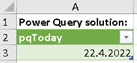
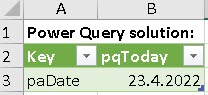
We will load this query into spreadsheet so that we have today's date in cell A3.
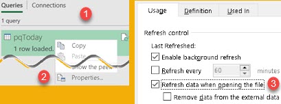
We will then set the option so that query is refreshed every time the file is opened.
In the pane with the queries (1), we should right click on our query and choose its Properties (2). In the new dialog we want to check option "Refresh data when opening the file" (3).
Possibility of error
There is a small problem with VBA and Power Query solutions. If we open the file just before a midnight, when the midnight pass, new day will arrive, but our date will not change. For VBA solution, we would need to enter the cell with F2 and press Enter ( F9 and Calculate Now would not work on UDF function ). For Power Query solution we would need to Refresh our query.
Closing and opening the file would also give us new date, or we can just turn off our computer and go to sleep before midnight.
Online Solution
Power Automate Solution
VBA and Power Query will not work for Excel online. We can use Power Automate to change date in one cell every day in midnight. We will combine Power Query solution and Power Automate solution, so that it doesn't matter if file is in cloud or on user's computer. First, we will change our query because Power Automate needs one more column. We are going to add "Key" column to our Power Query table.
let
Source = #table( type table [ #"Key"=text, #"pqToday"=date ]
, { { "paDate", DateTime.Date(DateTime.LocalNow()) } } )
in
Source
Now we can create flow that will change date in cell B3 every day in midnight.
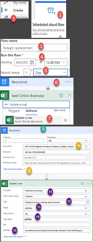
We click on "Create" button (1) for the new flow. Then we select "Scheduled cloud flow" (2). We will be offered dialog where we give our flow name (3), we can decide that from now, each day the flow will run (4,5). Next, we will get diagram view with "Recurrence" as the first step (6). As a next step we will add "Update a row" (7). Now that we have both our steps (8), we can fill necessary data.
In Recurrence step we just have to show advanced options (9) and decide what time zone should be used (10). In "Update a row" step we have to write where is our file and what is its name (11,12). (13)is the name of the declared table in which we are going to insert today's date. "Key" column is considered as primary key column so we have to give a value for primary key which defines row where we want changes to happen (14).
Name of declared table is "pqToday".
That row is made of fields. Those fields will appear at the bottom (15). We have only one field to fill. In this field we will write: convertFromUtc(utcNow(),'Central Europe Standard Time','dd.MM.yyyy'). This code will take current date according to given time zone and it will format it. This date will be written to our Excel file in cell B3.
For some reason step "Update a row" wasn't able to find my Excel file when I was using XLSM extension. It seams that file has to be XLSX.
An observational unit is the person or thing on which measurements are taken. Observational units have to be distinct and identifiable. Observational unit can also be called case, element, experimental unit or statistical unit. Examples of observational units are students, cars, houses, trees etc. An observation is a measured characteristic on an observational unit.
All observational units that have one or more characteristics in common, are called population. For example, if we observe people, all the people in one country can make population. They are all sharing the same characteristic that they are residents of the same country. One observational unit can belong to several populations at the same time, depending on the characteristics used to define those populations.
Sample is a subset of population units.
Population is a set of elements that are object of our research. Sampling is observing only subset of the whole population. Sample is always smaller then population, so it is really important for sample to be representative, it should have the same characteristics as the population.
Parameter is a function, that uses observations of all units in population, to calculate one real number. That real number represents value of some characteristic of the whole population. For example, if we have measured height of all the people in one population, we can use function μ = ( Σ Xi ) / N, to calculate average height. For specific given population, parameter is a constant that is result of parameter function.
Statistic is the same as Parameter, but it is calculated on a sample. Example would be function x̄ = ( Σ xi ) / N. When statistics is used as an estimate for a parameter, it is referred as an estimator.
Method (random, stratified, cluster…) used to select the observation units from a population into sample is known as sampling procedure. When we decide what sampling procedure and what statistics to use in our research, those two decision together created our sampling design.
For some sampling procedures we need to create list of all observation units that comprise that population. Such list is called frame or sampling frame.
Benefits and disadvantages of sampling
Benefits of sampling are: – Research can be conducted faster and with smaller cost. Organizational problems could be avoided. – Sometimes it is not possible to observe whole population. Some observational units are not accessible, or there is not enough highly trained personnel of specialized equipment for data collection. Sometimes we don't have enough time to observe full population. – When sample is smaller, personnel can be better trained to produce more accurate results. – Personnel could dedicate more time to one observational unit. They can measure many characteristics of a unit, so data can be collected for several science projects at the same time.
Collection of information on every unit in the population for the characteristics of interest is known as complete enumeration or census. Census would give us correct results. If we use sampling we can make mistakes like: – Our results could be biased. This is consequence of the wrong sampling procedure. – If phenomena under study is complex, it is really hard to select representative sample. Some inaccuracy will occur. – Sometimes it is impossible to properly collect the data from observation units. Some respondents will be not reachable, they will refuse to respond or they are not capable of responding. This would force us to find replacements for some observation units. – Sampling frame could be incorrect and incomplete. This is often the case with voters list.
Steps in sampling
Define the population. The definition should allow researcher to immediately decide whether some unit belongs to population or not.
Make a sampling frame.
Define the observation unit. All observation units together should create population. Observation units should not be overlapping, they should be exclusive.
Choose a sampling procedure.
Determine the size of a sample based on sampling procedure, cost, and precision requirements.
Create a sampling plan. Sampling plan is detailed plan of which measurements will be taken, on what units, at what time, in what way, and by whom.
Select the sample.
Types of sampling procedures
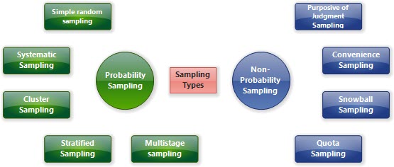
There are two groups of sampling methods. Those are Probability Sampling and Non-Probability Sampling. – Probability Sampling involves random selection where every element of the population has an equal chance of being selected. If our sample is big and randomly selected that would guarantees us that our sample is representative. Unfortunately, this is not so easy to accomplish. – Non-Probability Sampling involves non-random selection where the chances of selection are not equal. It is also possible that some units have zero chance to be included in the sample. We use this method when it is not possible to use Probability Sampling or when we want to make sampling more convenient or cost effective. Such sampling methods are often used in preliminary stages of research.
Probability Sampling procedures
Simple Random Sampling
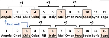
Simple random sampling requires that a list of all observation units be made. After this, we select some of observation units from that sampling frame by using either lottery technique or random numbers generator.
Sampling frame should be enumerated so that we can use five random numbers to select five Countries from our frame above.
Advantages of Simple Random Sample are: – It is simple to implement, no need for some special skills. – Because of its randomness, sample will be highly representative.
Disadvantages of Simple Random Sample are: – It is not suitable for large populations because it requires a lot of time and money for data collection. – This method offers no control to researcher so unrepresentative samples could be selected by chance. This method is best for homogenous populations where there is smaller risk to create biased sample. This could be solved only by bigger samples. – It could be difficult to create sampling frame for some population. – This method doesn't take in account existing knowledge that researcher has about population.
Systematic Sample
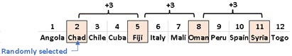
Systematic sample asks for population to be enumerated. If population has 12 units, and the size of sample is 4, we want to select one observation unit in every three (=12/4) consecutive units. The first element should be randomly selected in the first three observation units. We will select element 2 in our image below. After this, we will select every third unit. At the end, units 2,5,8 and 11 will create our sample.
In Systematic Sample first unit is randomly selected and others are selected in regular intervals.
Two other possible samples could start on first and on third element.
Advantages of Systematic Sample are: – Systematic Sample is simple and linear. – Chance of randomly selecting units that are close in population is eliminated. – It is harder to manipulate sample in order to get favored result. Systematic Sample rigidly decide which units will become part of a sample and which will not. This is only true if we have some natural order of units. If researcher can manipulate how units are ordered, then it could be actually easier for him/her to manipulate results.
Disadvantages of Simple Random Sample are: – We have to know in advanced, how big is our population, or at least we have to estimate its size. – If there is a pattern in units order, Systematic Sample will be biased. For example, if we choose every 11-th player in some football cup, we could actually select only goalkeepers. No regular player would be selected. We should avoid populations with periodicity.
Cluster Sampling
Cluster Sampling can be used when whole population could be divided into groups where each group has the same characteristics as the whole population. Such groups are called clusters. We can randomly select several clusters and they will comprise our sample.
Imagine that we want to investigate trees in some forest. We don't have to encompass all the trees. We can divide forest into parcels. We can then select several parcels and only trees in those parcels will be object of our research.
Advantages of Cluster Sampling are: – Observation units could be spatially closer to each other. In our example, all the trees on one parcel are in proximity of each other. This could significantly reduce cost of data collection. – Because observation units are close to each other it is easier to create and collect bigger samples. – If clusters really represent population, estimates made with cluster sampling will have lower variance.
Disadvantages of Cluster Sampling are: – We have to be careful not to include clusters that are different then general population. – Units shouldn't belong to several clusters. In our example, one tree can be on the border between parcels. We could measure it twice. – It is statistical requirement that all clusters should be of similar size.
Stratified Sampling
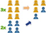
Stratified Sampling involves dividing the population into subpopulations that may differ in some important trait. Such subpopulations should not overlap and together they should comprise the whole population. One such subpopulations is called stratum. Plural of the word stratum is strata. After this, we should take simple random of systematic sample from each stratum. Number of units taken from each stratum should be proportional to the size of the stratum.
Here, we divided our population based on gender. In our population ratio between men and women is 3:2. The same ratio should stay inside of our sample. If our population has 6 women and 4 men, then our sample should have 3 women and 2 men, if the size of sample is 5 in total.
Advantages of Stratified Sampling are: – Every important part of population is included in sample. – It is possible to investigate differences between stratums. – Because units in each strata are similar, average value of some characteristic of those units will have smaller variance. This will have as consequence that variance of estimator for the whole population will have smaller variance too.
Disadvantages of Stratified Sampling are: – We need to make complete sampling frame. Each observation unit has to be classify in which stratum belongs. – Often it is hard to divide population in subpopulations that are internally homogenous but are heterogenous between them.
Multistage Sampling
Multistage Sampling is a method of obtaining a sample from a population by splitting a population into smaller and smaller groups and taking samples of individuals from the smallest resulting groups. Multistage Samplinginvolves stacking multiple sampling methods one after the other. Stratified Sampling is a special case of Multistage Sampling because it has two stages. One other possible method could be to divide population into clusters and then to take systematic sample from each cluster.
Non-Probability Sampling procedures
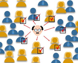
Purposive of Judgment Sampling
Judgmental sampling is when the researcher have right to discretely selects the units of the sample, by using their knowledge. It is used when researcher wants to gain detailed knowledge about some phenomenon. It is also used when population is very specific and hard to identify.
You want to interview winners of lottery about how they are spending and investing their money. Well, there are not so many winners of lottery and many of them will refuse to speak with researcher or their identity is a secret. Examiner will not find many people to talk with. In that case, every winner willing to share their experience will become part of purposive sample.
Another example would be when researcher interview only people who gave the most representative answers in some previous research or he/she wants to interview only people which have enough knowledge to predict some future event.
Advantages of Purposive Sampling are: – It can be used for small and hidden populations. – Examiner can use all of his knowledge to create heterogenous and representative sample. – This sampling method can combine several qualitative research designs and can be conducted in multiple phases.
Disadvantages of Purposive Sampling are: – There is huge bias because sample is not selected by chance. Also, when we use purposive sampling, our sample is usually small. – There is no way to properly calculate optimal size of sample or to estimate accuracy of the research results. – Examiner can easily manipulate the sample to get artificial results.
Convenience sampling
In this sampling procedure, units are selected based on their availability and willingness to take part. Studies that rely on volunteers or studies that only observe people on convenient places like busy streets, malls or airports are examples of Convenience Sampling. This technique is known as one of the easiest and cheapest.
Advantages of Convenience Sampling are: – We can collect answers from dissatisfy buyers or employees. People are hesitant to express their dissatisfaction openly but they are more willing to do it during some research. – This method is good for first stages of research because we don't have to worry about quality of our sample, all participants are willing to give us answers, we can collect some demographic data about them, we can get immediate feedback. – It is cheap and fast.
Disadvantages of Convenience Sampling are: – Potential bias. We are only covering people and things near to us, all others will be neglected. Results from convenience sampling can not be generalized. – People who are in a hurry will often give us incomplete or false answers to shorten the interaction with us. This can cause the examiner to start avoiding people who are nervous or in a hurry and thus further reduce the representativeness of the sample.
Snowball Sampling
For Snowball Sampling we have to start with only few participants. Those people are asked to nominate further people known to them so that the sample increases in size like a rolling snowball. This technique is needed when participants don't want to talk about their situation because they feel vulnerable or in danger. Such populations are homeless, illegal immigrants, people with rare diseases.
Advantages of Snowball Sampling are: – It can be used when sampling frame is unknown, when respondents don't want to disclose their status or to identify themselves. – Sampling process is faster and more economical because existing contacts are used to reach to other people.
Disadvantages of Snowball Sampling are: – Because they are connected, all participants have some common traits. This can exclude all other members of our population who don't share those traits. This means that there is huge bias in our research because population is not correctly presented. – People from vulnerable groups can show resistance and doubt. Researcher has to be careful to earn their trust. – Examiner can not use his previous knowledge to make sample better. He can not control the sampling process.
Quota sampling
Quota Sampling is similar to stratified sampling. Here, we also try to split population in exclusive homogeneous groups. This way we reduce variance inside such groups. After this, we apply some non-probability sampling method to select units inside our strata.
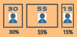
We don't know how big is our population, nor do we know how big are strata. Instead of that we are trying to guess what percentage of general population makes each of strata, based on some older research or on our expertise. We also have to decide how big our sample should be. Because samples from each stratum should be proportional to stratum size, we have enough information to decide how many units to pick from each stratum. If our strata are in proportion of 30% : 55% : 15%, and we want sample of 100 units then we have to choose 30, 55, 15 units from each stratum respectively.
Advantages of Quota Sampling are: – Quota Sampling is simpler and less demanding on resources, similar to other non-probability sampling methods. – Scientist can increase precision of research by proper segmentation of population by using his knowledge. – We don't need to have sampling frame.
Disadvantages of Quota Sampling are: – Like other non-probability methods, Quota Sampling introduce bias but that could be mitigate by proper partition of population.
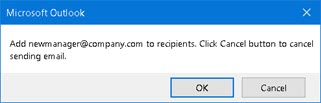
This post will explain how to use VBA to get a reminder each time you try to send email with specific words in its subject. Let's say you have a mail with a subject "New products". You send this email every month. Someone informs you that, the next time when you send this email, you have to add "newmanager@company.com" to a list of recipients. Usually you would just hit "Replay All" button on the old email, make some changes, and then you would send newly made email. But, it is very hard to recall, in that specific moment, to add the new manager to recipient list. It would be great to get message like this that would remind us of a needed change.
VBA procedure
We can use VBA procedure to reminds us to make a change. In the sample files, at the end of this blog post, you will find such VBA procedure. This procedure has to be placed in the Outlook VBA environment in ThisOutlookSession. This procedure has hardcoded array that looks like this:
Array(Array("New", "products"), "Add newmanager@company.com to recipients. Click Cancel button to cancel email.")
What this array says is to look for an email that has both "New" and "products" words in its subject. Array could have as many searched words as we want. We will change this procedure by placing our searched terms in it. This is how we say to VBA procedure what are we looking for. After this first step, don't close your Outlook, we have to solve certification problem.
Certification problem
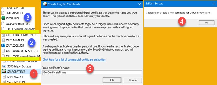
Outlook should always have macro security turned on. This, unfortunately means that our macro will be either disabled or we will get notifications each time we open Outlook. The only way out is to acquire a digital certificate. You can buy such certificate or you can create your own with "SelfCert.exe" program. It is not common to buy your own digital certificate so most people will use the one made with "SelfCert.exe". This is small program which is included in every Windows. Certificate created with it will be only valid for computer on which that certificate is created. This is enough to make our reminder VBA procedure fully operational.
We can find "SelfCert.exe" (1) in the same folder where Excel and Outlook are placed (2,3). When we find this program, we click on it and the window (3) is opened. Here, we have to give our certificate a name. After this, confirmation message is shown(4). This is how we create certificate.
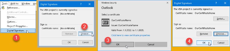
Now we have to implement our certificate in Outlook. We go to VBA environment, and in Tools menu we choose "Digital Signature" option (1). New dialog will open. In it, we click on "Choose" button (2). Now, we will be offered with our previously created certificate and we will accept it (3). We return to dialog (4) again where we click on OK button.
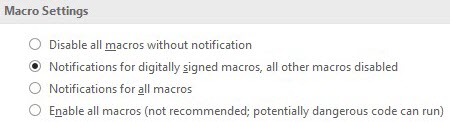
Before closing Outlook, make sure that your macro security level is set to "Notifications for digitally signed macros, all other macros disabled".
After this, our VBA procedure is placed in correct place and it is certified. We can close Outlook now. We will get a confirmation dialog to save VBA project which we will confirm.
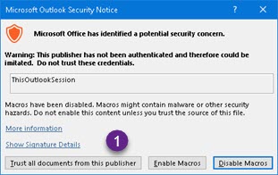
Sending an email
Open Outlook. Before fully open, Outlook will show us a message (1). On this message we have to click on "Trust all documents from this publisher". We have to do this only once.
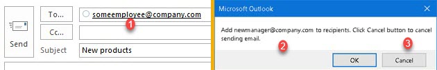
Only now, can we try our VBA procedure. When we try to send email (1) with subject that has words "New" and "products", instead we will get a message box (2) with notification "Add newmanager@company.com to recipients. Click Cancel button to cancel email.".
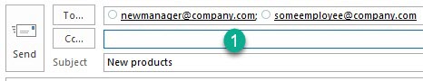
If you click on Cancel (3), message box will close but email will not be send. Now, we can change recipient list. We can add "newmanager@company.com" to our mail (1).
After our mail is corrected, we will delete our Array from VBA procedure. Then we can send our email normally.
We can have several such arrays. Each array is a trap waiting for your email to be send. First trap to catch your email will decide what message to show to the user. If no traps catch something, that email will be send without notification.
Array( Array("New", "products"), "Add newmanager@company.com to recipients. Click Cancel button to cancel email.") _
, Array( Array("New", "and", "old"), "Add newemployee@company.com to recipients. Click Cancel button to cancel email.")
Problem with creating certificate
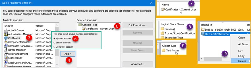
Sometimes we will have problem to create our certificate with "SelfCert.exe" program. We can try to delete our old certificates. Go to Run > mmc (1). In new dialog, click on File > Add/Remove Snap-in (2).
Sub dialog will then open. Select "Certificates" (3) and add them (4,5) into pane (6). Now, close sub dialog and return to the main dialog. There, click on "Certificates – Current User" (7), then on "Personal" (8), and finally on "Certificates" (9). Here, you will see your certificate and you can delete it (10).
Also, go to location "C:\Users\<yourUsername>\AppData\Roaming\Microsoft\Crypto\RSA" and there delete all of the subfolders.
Finally, reset your computer. You should now be able to create new certificate with SelfCert.exe.
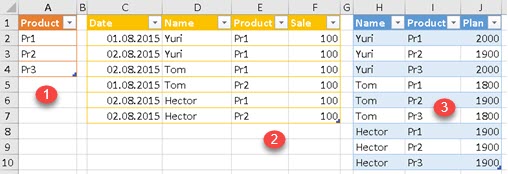
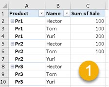
We have three tables below. Table (1) shows all products we sell. Table (2) shows our sale in first two days of a month. Note that we still didn't have sale for Product 3 in that month. In third table (3) we have month plan defined for each Salesman/Product combination.
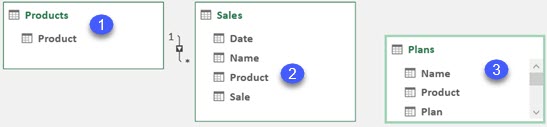
In our model we will connect the first (1) and the second (2) table with a relation. Plan (3) will be detached table and we will use measure to get our plan values.
"Show items with no data on rows" pivot table option
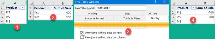
If we add column Products[Product] into pivot table (1), all three products will be shown. After we add column Sales[Sale] to the same pivot table, only two products will remain (2). This is consequence of the fact that we didn't have any Product 3 sales. This behavior could be changed by enabling option "Show items with no data on rows" (3) in the pivot table options. Now, we can see that all the three products are presented (4).
Problem description
We will start with a pivot table (1) below. Option "Show items with no data on rows" is enabled. This pivot table has no Grand Total in order to make things simpler. Then, we will create measure [Target](2) which will add Plans[Plan] values into our pivot table. This measure will use DISTINCT function. As we can see, rows 7-10 in image (3)will have no plan values, although we have them defined. The reason for this is in the expression DISTINCT( Sale[Name] ). This expression will return BLANK() for each row where [Sum of Sale] is also BLANK(). That is consequence of the fact that in Sales table there are no rows with Product/Name combinations like in rows 7-10. DISTINCT function is trying to read directly from table Sales, but there are no rows to read from.
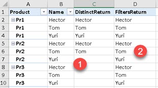
Instead of DISTINCT function, we should have used FILTERS function. This function accepts only one column argument. It returns all of values that are filtered from that column. Let's make two simple measures "DistinctReturn:=DISTINCT( Sales[Name] )" and "FiltersReturn:=FILTERS( Sales[Name] )" to see difference between them.
DISTINCT (1) will not return anything for rows 7-10 as we saw earlier. FILTERS (2) function will return "Yuri" in cell "D7" because column Sale[Name] is filtered by only that value in that specific row. That is why column [FiltersReturn] has result in each row, because it is reading filter context for column Sales[Name], and is not reading from Sales[Name] column itself. Column Sales[Name] is reduced to nothing in cell "C7" because there are no rows with "Pr2 & Yuri" combination in the Sales table.
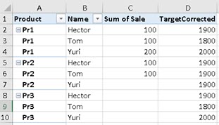
Now, that we know, what is the problem, we can create correct expression for Target measure. We only need one small change. We have to replace DISTINCT with FILTERSfunction to get correct result.