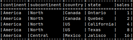
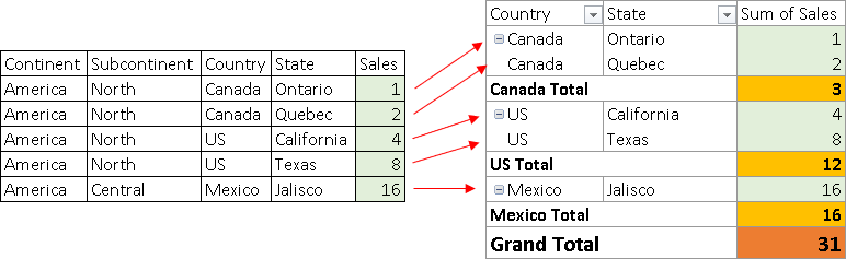
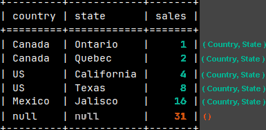
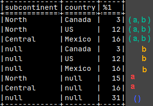
When we create a Pivot table, from the sample table, we will see all of the detail sales (1,2,4,8,16), but we will also see totals (3,12,16,31).
The question is, what query would return all of these numbers, both detail values and totals, if we use MonetDB.
This is one possible solution:
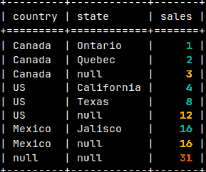
SELECT Country, State, Sales FROM tabSales UNION ALL SELECT Country, null, SUM( Sales ) FROM tabSales GROUP BY Country UNION ALL SELECT null, null, SUM( Sales ) FROM tabSales;
On the image, the rows are sorted so that the table looks like the pivot table.
UNION ALL solution is bad for several reasons: 1) We have three queries to execute and then to combine multiple result sets into one. 2) It is hard to read and modify long UNION ALL query. 3) We have to be careful to properly align columns.
This is the problem that can be solved by grouping sets.
Grouping Sets
"Grouping Sets" are much better and faster syntax to achieve the same goal.
SELECT Country, State, SUM( Sales )
FROM tabSales
GROUP BY GROUPING SETS ( Country, State, ( ) );
Empty parentheses are for the grand total.
We'll get the same result, except the repetition of country names is reduced. Instead of them we have nulls.
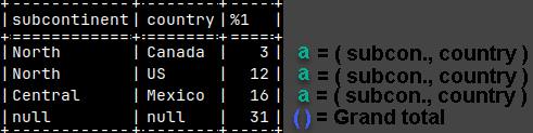
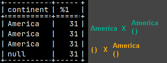
Look what we will get if we place parentheses around Country and State.
SELECT Country, State, SUM( Sales )
FROM tabSales
GROUP BY GROUPING SETS ( ( Country, State ), () );
Parentheses are there to define each group.
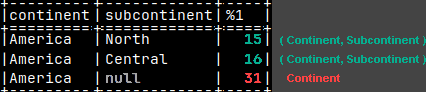
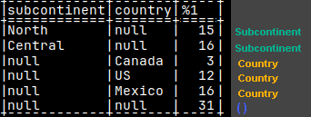
We can see the effect of parentheses better on this example.
SELECT Continent, Subcontinent, SUM( Sales )
FROM tabSales
GROUP BY GROUPING SETS ( ( Continent, Subcontinent ), Continent );
Continent can be used by itself, but it can be also used in conjunction with Subcontinent to define a group.
It is now clear that each element, inside GROUPING SETS, is a separate definition of a group. Each group can be defined by one column > Continent <, or by several columns placed inside of the parentheses ( Continent, Subcontinent ).
These two examples, that would return the same result, show the logic and brevity of the grouping sets.
SELECT Col1, Col2, SUM( Sales )
FROM Table
GROUP BY GROUPING SETS
    (  ( Col1, Col2 ), Col1 );
SELECT Col1, Col2, Sales FROM Table
UNION ALL
SELECT Col1, null, SUM( Sales ) FROM Table GROUP BY Col1;
Rollup
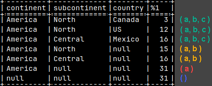
SELECT Continent, Subcontinent, Country, SUM( Sales )
FROM tabSales
GROUP BY ROLLUP( Continent, Subcontinent, Country );
ROLLUP( a, b, c ) is the same as grouping sets "( a, b, c ), ( a, b ), ( a ), ()". This is a way to get hierarchy of the columns. Rollup will give us all of the numbers that we need to create a pivot table.
For ROLLUP, the order of the columns is important.
ROLLUP( a, b, c )                ROLLUP( c, b, a )

( a, b, c )                      ( c, b, a )
( a, b )                         ( c, b )
( a )                            ( c )
( )                              ( )
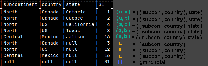
Similar to GROUPING SETS, ROLLUP can also create combinations of columns by using parentheses.
SELECT Subcontinent, Country, State, SUM( Sales )
FROM tabSales
GROUP BY ROLLUP( ( Subcontinent, Country ), State );
CUBE
CUBE works similar to ROLLUP, but have a different logic. CUBE will give us all of the possible combinations. CUBE( a, b, c ) will give us 2^3 grouping sets "(a,b,c), (a,b), (a,c), (b,c), (a), (b), (c) and ()". ———————————————————————————-
SELECT Subcontinent, Country, SUM( Sales ) FROM tabSales GROUP BY CUBE( Subcontinent, Country ); Because we have only 2 columns inside of CUBE in our example, number of combinations is 2^2 = 4 "(a,b), (b), (a), ()".
We can also define groups by using parentheses. SELECT Subcontinent, Country, SUM( Sales ) FROM tabSales GROUP BY CUBE( ( Subcontinent, Country ) ); We now have only one element. We have only two ( 2^1 ) groups "(a), ()".
Addition and Multiplication in Grouping Sets
This is addition: ( a, b ) + ( c ) = ( a, b ) ( c )
This is multiplication. Multiplication is crossjoin between individual values. a1bc1 ( a ) ( b, c ) a1bc2 a1 * bc1 = a1bc3 a2 bc2a2bc1 bc3a2bc2 a2bc3
Syntax for addition is like this. Everything inside of the GROUPING SETS parentheses will be added to each other. In this example we will add ( Subcontinent ) + ( Country ) + ( ).
SELECT Subcontinent, Country, SUM( Sales )
FROM tabSales
GROUP BY GROUPING SETS ( Subcontinent, ROLLUP( Country ) );
So, if we create GROUPING SETS like this, this will be addition. GROUPING SETS ( Continent, ROLLUP( Continent, Subcontinent ), CUBE( Country, State ), () )
Addition can easily create duplicates: SELECT Continent, SUM( Sales ) FROM tabSales GROUP BY GROUPING SETS ( CUBE( Continent ), () );
CUBE will create Grand Total, but we will also get grand total from the "( )" element.
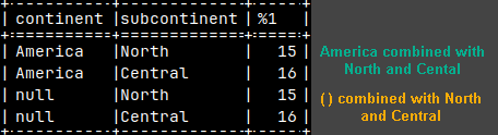
This is a syntax for multiplication. This time we will have commas between GROUPING SETS, ROLLUPS and CUBES, and individual elements. GROUPING SETS ( Continent ), ROLLUP( Continent, Subcontinent ), CUBE( Country, State ), (),Country
This example will give us 2 x 2 = 4 rows. ROLLUP will give us America, and "( )". GROUPING SETS will give us "North" and "Central". Then we combine them 2 x 2.
SELECT Continent, Subcontinent, SUM( Sales ) FROM tabSales
GROUP BY ROLLUP( Continent ), GROUPING SETS ( Subcontinent );
Multiplication can also easily create duplicates: SELECT Continent, SUM( Sales ) FROM tabSales GROUP BY GROUPING SETS ( Continent, () ), GROUPING SETS ( Continent, () );
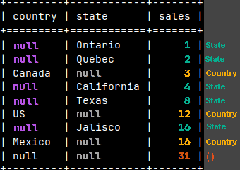
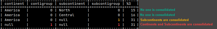
Indicator Function – GROUPING
GROUPING function will inform us what rows are subtotals / grand total. In such rows, some columns have nulls because they are consolidated. GROUPING function has an argument which is a column, and GROUPING function will return the result only for that column.
SELECT Continent, GROUPING( Continent ) AS ContiGroup, Subcontinent, GROUPING( Subcontinent ) AS SubcontiGroup , SUM( Sales )
FROM tabSales
GROUP BY ROLLUP ( Continent, Subcontinent );
This function is important because it help us to make distinction between subtotal nulls, and missing data nulls.
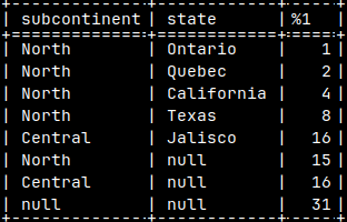
Formatting with COALESCE and Sort
This is not good looking table. Let's fix it.
SELECT Subcontinent, State, SUM( Sales )
FROM tabSales
GROUP BY ROLLUP( Subcontinent, State );
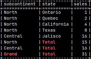
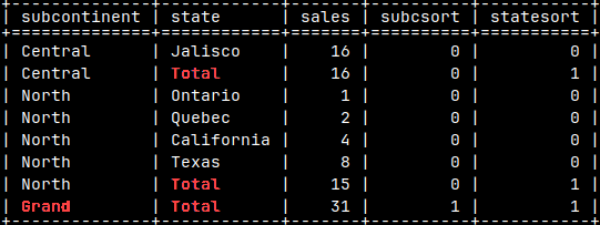
COALESCE will helps us to eliminate NULLS: SELECT COALESCE( Subcontinent, 'Grand' ) AS Subcontinent , COALESCE( State, 'Total' ) AS State , SUM( Sales ) AS Sales FROM tabSales GROUP BY ROLLUP( Subcontinent, State );
With GROUPING function, we can create columns that will help us to sort the table.
SELECT COALESCE( Subcontinent, 'Grand' ) AS Subcontinent
      , COALESCE( State, 'Total' ) AS State
      , SUM( Sales ) AS Sales
      , GROUPING( Subcontinent ) AS SubcSort
      , GROUPING( State ) AS StateSort
FROM tabSales GROUP BY ROLLUP( Subcontinent, State )
ORDER BY SubcSort, Subcontinent, StateSort;
These auxiliary columns ( SubcSort and StateSort ) can be easily eliminated by wrapping everything with "SELECT Subcontinent, State, Sales".
Comments
Sample Table and Function
Let's create two tables and function.
CREATE TABLE tabComment( Number INTEGER );
CREATE TEMPORARY TABLE tabTemporary( Number INTEGER );
CREATE OR REPLACE FUNCTION funcComment( Arg1 INTEGER )
RETURNS INTEGER
BEGIN
     RETURN 2;
END;
Comments on Database Objects
We can create comments that are tied for database objects. Comments convey information about that object.
COMMENT ON TABLE tabComment IS 'tabComment description'; COMMENT ON COLUMN tabComment.Number IS 'Number column description'; COMMENT ON FUNCTION funcComment IS 'funcComment description'; COMMENT ON SCHEMA sys IS 'sys schema description';
We will then find IDs of our database objects: SELECT * FROM sys.tables WHERE name = 'tabcomment'; 15876 SELECT * FROM sys.columns WHERE table_id = 15876; 15875 SELECT * FROM sys.functions WHERE name = 'funccomment'; 15881 SELECT * FROM sys.schemas WHERE name = 'sys'; 2000
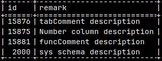
All of these IDs can be found in the system table "sys.comments" together with their comments. SELECT * FROM sys.comments WHERE Id IN ( 15876, 15875, 15881, 2000 );
Deleting a Comment
If we delete an object, its comment will be deleted. DROP TABLE tabComment; SELECT * FROM sys.comments WHERE Id = 15876;
We can delete a comment by setting it to NULL or an empty string. COMMENT ON SCHEMA sys IS null; SELECT * FROM sys.comments WHERE Id = 2000;
If a function is overloaded then we have to provide the full signature. COMMENT ON FUNCTION funcComment( INTEGER ) IS ''; SELECT * FROM sys.comments WHERE Id = 15881;
Persistent Database Objects
There are other database objects that we can place a comment on. They are all persistent database objects.
COMMENT ON VIEW view_name IS 'Comment';
COMMENT ON INDEX index_name IS 'Comment';
COMMENT ON SEQUENCE sequence_name IS 'Comment';
COMMENT ON PROCEDURE procedure_name IS 'Comment';
COMMENT ON AGGREGATE aggregate_name IS 'Comment'; COMMENT ON LOADER loader_name IS 'Comment';
We can not create a comment on a temporary object. COMMENT ON TABLE tabTemporary IS 'tabTemporary description';
Note: Before reading this blog post, you should read article about merge tables in the MonetDB ( article ), or you can watch on youtube ( video ). Advice: I suggest you follow this blog as a strict instruction. Any freestyling could mean that you will have problems to create remote tables.
Visual Presentation
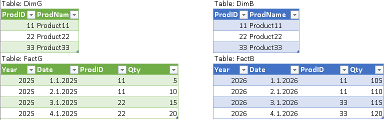
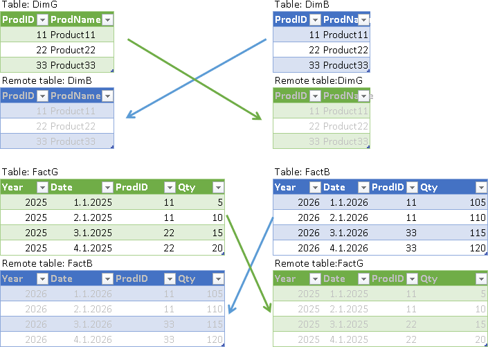
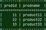
In this case, we will use two MonetDB instances that are placed on two different computers. Both of them will have dimension table with products, and that table will have the same data on both computers (DimG and DimB on the image). I will use (G)reen and (B)lue colors to differentiate servers.
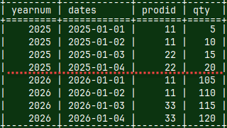
Fact table will be divided into two parts. FactG will be on the green server, and FactB will be on the blue server. They will have different data.
The next step is to create remote tables. Remote tables are references on one server to tables on another server. The purpose of remote tables is to let each server know about all of the tables in the system and how those tables are connected. This allows each server to create a query execution plan, even though that query uses tables from both servers.
Green server
Blue server
Table: DimG Remote table: DimB
Table: FactG Remote table: FactB
Table: DimB Remote table: DimG
Table: FactB Remote table: FactG
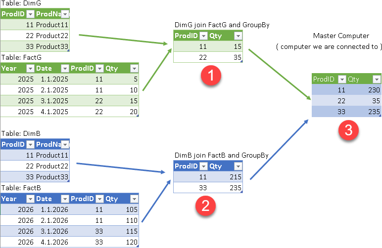
As a user, we can now connect to one server (it doesn't matter which one) and we can execute a query that will use tables from both servers.
The computer we connect to will create an execution plan for the query. This plan will usually assume that intermediate results (1,2) will be calculated on each server. That way we can divide processing between the servers and increase parallelism.
The intermediate results will then be collected by the master computer (the one that creates the execution plan) and transformed into the final result (3).
The whole purpose of distributed queries is to divide the work between the computers in the cluster and increase performance.
In this part, we will create MonetDB folder, one database, and we will login as administrator.
As admin we will create new role, schema and user. Schema will have that role as authorization. User will have that schema as default schema, and role as default role. That means that user will be able to use all of the objects in this schema.
CREATE ROLE RoleGB;
CREATE SCHEMA SchemaGB AUTHORIZATION RoleGB;
CREATE USER UserGB WITH PASSWORD 'gb' NAME 'Distributed User' SCHEMA SchemaGB DEFAULT ROLE RoleGB;
quit
Letters "GB" mean that this role, schema and user will exist in both the green and the blue server. In order for one user to access tables from both servers, his account must be present in both servers.
Then, we will login as a new user "usergb". We will create two tables, "DimG" and "FactG", and we will fill them with the data.
At the start of this blog post, we already saw content of these tables.
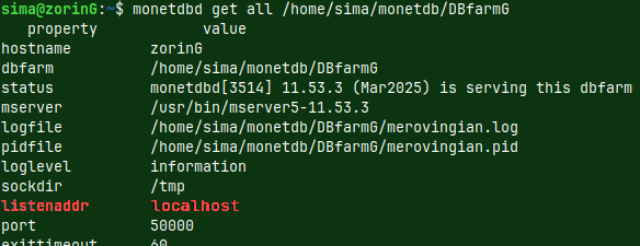
monetdbd stop /home/sima/monetdb/DBfarmG
monetdbd get all /home/sima/monetdb/DBfarmG
monetdbd set listenaddr=0.0.0.0 /home/sima/monetdb/DBfarmG
We are back in the shell. I will stop monetdb folder because I want to change one setting. That setting is "listenaddr". This setting is currently "localhost" which means that server is only available from the local computer.
We will change that value to "0.0.0.0" which means that anyone can access MonetDB server.
We will then start our MonetDB folder again: monetdbd start /home/sima/monetdb/DBfarmG
We can test who is listening the port 50.000. ss -tulnp | grep 50000
Below you can see some commands that you can use to configure your firewall so that you can control communication between servers. I will not teach you how to manage the firewall. I will just show you how I configured it. If you have any problems with the firewall, you can reset all the rules with "sudo ufw reset", and then you can disable the firewall with "sudo ufw disable".
I will now set firewall by running these commands in the shell.
"ufw" means "uncomplicated firewall".
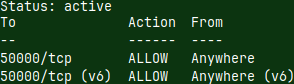
sudo ufw enable --the firewall will be permanently enabled. It is disabled by default. sudo ufw default deny incoming --no one can call us sudo ufw default allow outgoing --we can call anyone -- bellow is command that will open incoming traffic on port 50.000 for tcp protocol. -- it will also limit the range of IP addresses only to IP addresses on my local network. sudo ufw allow from 192.168.100.0/24 to any port 50000 proto tcp -- I don't know whether your local network is using the same range of IP addresses. I will delete this rule. sudo ufw delete allow from 192.168.100.0/24 to any port 50000 proto tcp --I will create a simpler rule that will only limit the port number and tcp protocol. sudo ufw allow 50000/tcp sudo ufw status --we can check the status of the firewall.
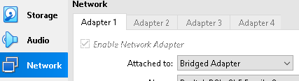
This step is just for the people who are following this tutorial with linux virtual machines inside of the Virtual Box. Go to Settings > Network > Adapter 1, and choose the "Bridged Adapter" option. This will include virtual machines into the local network. This step is needed so that two virtual machines can communicate over the network.
Testing Remote Access to the Green Server
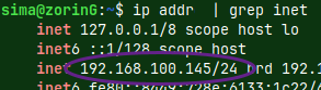
In the green server shell, run this command. This is how you can find IP address of a server. ip addr | grep inet
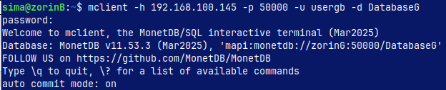
Now you can go tothe blue server, and from there you can run this code. mclient -h 192.168.100.145 -p 50000 -u usergb -d DatabaseG -- password is "gb" This is how we can log to remote green server, over the network.
Blue Server Setup
There is nothing different in preparing of the blue server. I will just repeat the same commands, but with different identifiers.
CREATE ROLE RoleGB; --all identifiers are the same for the privileges, as for the green server CREATE SCHEMA SchemaGB AUTHORIZATION RoleGB; CREATE USER UserGB WITH PASSWORD 'gb' NAME 'Distributed User' SCHEMA SchemaGB DEFAULT ROLE RoleGB; quit;
mclient -u usergb -d DatabaseB --now we login as the user CREATE TABLE FactB ( YearNum INT, Dates DATE, Prodid INT, Qty INT ); INSERT INTO FactB VALUES (2026, '2026-01-01', 11, 105), (2026, '2026-01-02', 11, 110) , (2026, '2026-01-03', 33, 115), (2026, '2026-01-04', 33, 120); CREATE TABLE DimB ( ProdID INT, ProdName VARCHAR(50) ); INSERT INTO DimB VALUES (11, 'product11'), (22, 'product22'), (33, 'product33'); quit
monetdbd stop /home/sima/monetdb/DBfarmB monetdbd get all /home/sima/monetdb/DBfarmB monetdbd set listenaddr=0.0.0.0 /home/sima/monetdb/DBfarmB --we make the server available from the network monetdbd start /home/sima/monetdb/DBfarmB ss -tulnp | grep 50000
sudo ufw enable --if needed, we can set firewall sudo ufw default deny incoming sudo ufw default allow outgoing sudo ufw allow 50000/tcp sudo ufw status
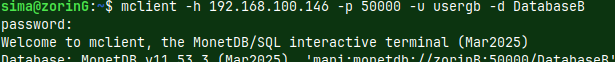
We can login to blue server from the green server (password="gb"). mclient -h 192.168.100.146 -p 50000 -u usergb -d DatabaseB
Preparing REMOTE, REPLICA and MERGE Tables in the Green Server
In the green server, we will create REMOTE tables that are just references toward tables in the blue server. mclient -u monetdb -d DatabaseG --only admin can create REMOTE tables (pass="monetdb") SET SCHEMA SchemaGB; --we must be in the same schema as the physical tables in the blue server CREATE REMOTE TABLE DimB( ProdID INT, ProdName VARCHAR(50) ) on 'mapi:monetdb://192.168.100.146:50000/DatabaseB'; --ip address of blue server CREATE REMOTE TABLE FactB( YearNum INT, Dates DATE, ProdID INT, Qty INT ) on 'mapi:monetdb://192.168.100.146:50000/DatabaseB';
CREATE REPLICA TABLE Dim( prodid INT, prodname VARCHAR(50) );
ALTER TABLE Dim ADD TABLE DimG;
ALTER TABLE Dim ADD TABLE DimB;
Tables "DimG" and "DimB" are totally identical. We must notify MonetDB that they are "replicas". For queries MonetDB can use any of these tables interchangeably.
CREATE MERGE TABLE Fact( YearNum INT, Dates DATE, ProdID INT, Qty INT );
ALTER TABLE Fact ADD TABLE FactG;
ALTER TABLE Fact ADD TABLE FactB;
Tables "FactG" and "FactB" are just partitions of the merge table. This is why you should read/watch video about merge tables.
We can now query these two new tables Dim and Fact.
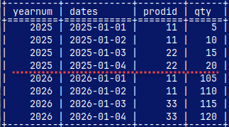
Dim table is unchanged, but Fact table is UNION of FactG and FactB.
SELECT * FROM Dim;
SELECT * FROM Fact;
Preparing REMOTE, REPLICA and MERGE Tables in the Blue Server
I will again repeat all of the steps, but this time for the blue server.
mclient -u monetdb -d DatabaseB --only admin can create REMOTE tables. (pass="monetdb") SET SCHEMA SchemaGB; --we must be in the same schema as the physical tables in the blue server CREATE REMOTE TABLE DimG( ProdID INT, ProdName VARCHAR(50) ) on 'mapi:monetdb://192.168.100.145:50000/DatabaseG'; CREATE REMOTE TABLE FactG( YearNum INT, Dates DATE, ProdID INT, Qty INT ) on 'mapi:monetdb://192.168.100.145:50000/DatabaseG';
CREATE REPLICA TABLE Dim( ProdID INT, ProdName VARCHAR(50) ); ALTERTABLE Dim ADD TABLE DimG; ALTER TABLE Dim ADD TABLE DimB;
For performance reasons, MonetDB does not check if the replica tables are indeed identical. This responsibility is left to the database users.
CREATE MERGE TABLE Fact( YearNum INT, Dates DATE, ProdID INT, Qty INT ); ALTER TABLE Fact ADD TABLE FactG; ALTER TABLE Fact ADD TABLE FactB;
SELECT * FROM Dim; SELECT * FROM Fact;
Horizontally dividing one table between computers in a cluster is called "sharding".
System Tables
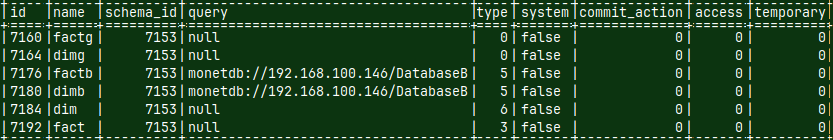
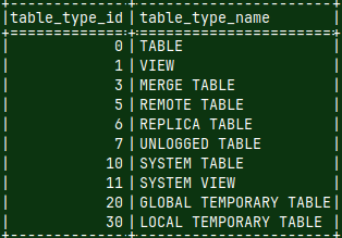
In "sys.tables" we can find all our tables. Based on the system table "sys.table_types" we can see that we have regular (0), remote (5), merge (3) and replica tables (6). SELECT * FROM sys.tables WHERE name IN ( 'factg', 'factb', 'fact', 'dimg', 'dimb', 'dim' );
SELECT * FROM sys.table_types;
Dependencies inside of "fact" and "dim" table can be seen in the system view "sys.dependencies_vw". SELECT * FROM sys.dependencies_vw WHERE depend_type = 2;
The Fruit of Our Labor
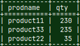
In the green server, I will now login as a "UserGB". This user has privileges over all of the objects in the "SchemaGB". He can query "Dim" and "Fact" tables. mclient -u usergb -d DatabaseG --password "gb" SELECT ProdName, SUM( Qty ) AS Qty FROM Dim INNER JOIN Fact ON Dim.ProdID = Fact.ProdID GROUP BY ProdName;
Finally, we can run a query that will use the power of the two computers and two MonetDB servers.
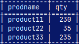
It is the same for the blue server. mclient -u usergb -d DatabaseB --password "gb" SELECT ProdName, SUM( Qty ) AS Qty FROM Dim INNER JOIN Fact ON Dim.ProdID = Fact.ProdID GROUP BY ProdName;
We finally have a working distributed query processing system.
Load Balancer
The question is how to divide users between two (or more) servers to equalize the load. The easiest way is to have all users born from January to June use the green server, and all users born from July to December use the blue server.
A more professional way is to use a load balancer, something like HAproxy (link). This program will direct users to a server that is currently not under load.
We will start with a blank state. I will delete the users that were created in the Part 1.
DROP USER newUser;
DROP USER mnm;
Initial State
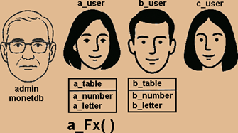
mclient -u monetdb -d voc #password "monetdb" I will create three users. I won't define their default schemes, so each of them will get a scheme named after them. We also have admin user "monetdb".
CREATE USER a_user WITH PASSWORD '1' NAME 'a';
CREATE USER b_user WITH PASSWORD '1' NAME 'b';
CREATE USER c_user WITH PASSWORD '1' NAME 'c';
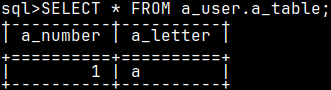
I will now login as "a_user" and I will create a table and a function. They will be created in the schema "a_user". mclient -u a_user -d voc #password "1" CREATE TABLE a_user.a_table ( a_number INT PRIMARY KEY, a_letter CHAR ); INSERT INTO a_user.a_table ( a_number, a_letter ) VALUES ( 1, 'a' );
CREATE OR REPLACE FUNCTION a_user.a_Fx()
RETURNS INTEGER
BEGIN
     RETURN 2;
END;
I will create one table in the "b_user" schema. mclient -u b_user -d voc #password "1"
Privilege is a permission to do one action (SELECT, UPDATE…). Role is a collection of such privileges.
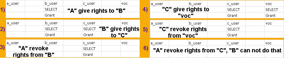
Grant Privileges to a User
Grant and Revoke all Privileges on a Table
"b_user" can not use the table "a_table".
"a_user" will grant privilege to "b_user" to use table "a_table". "FROM CURRENT_USER" is the default and can be omitted. That means that the privilege is given by the CURRENT_USER. Other option is that the privilege is given by a role. We'll see that later.
mclient -u a_user -d voc #password "1" GRANT ALL ON a_user.a_table TO b_user FROM CURRENT_USER;
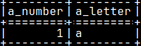
We will now log in as a b_user and we will try to use "a_table". mclient -u b_user -d voc #password "1"
SELECT * FROM a_user.a_table;
"b_user" can not alter the table. Altering of a table is reserved for an owner of a table. "b_user" can only use DML stataments. In MonetDB, owner of a table is owner of a schema where some table is.
ALTER TABLE a_user.a_table RENAME COLUMN a_number TO zzz;
mclient -u a_user -d voc #password "1" REVOKE ALL ON TABLE a_user.a_table FROM b_user;
This is how we can revoke privileges given to "b_user".
Grant and Revoke Separate Privileges
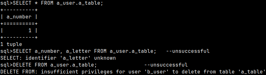
I will again give privileges to "b_user" for the table "a_table". GRANT SELECT ( a_number ), INSERT, UPDATE ( a_number, a_letter ) ON a_user.a_table TO b_user FROM CURRENT_USER; This time, instead of "ALL", I will give each privilege separately. This time I will give him SELECT, INSERT and UPDATE privileges. Beside those we can give him privileges to DELETE, TRUNCATE, and REFERENCE. Any combination is allowed. Notice that for SELECT, UPDATE and REFERENCES we can limit our permission to a list of columns.
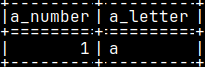
I will then login as a "b_user" and I will try SELECT and DELETE on "a_table". mclient -u b_user -d voc #password "1" SELECT * FROM a_user.a_table; --successful, but only 1 column SELECT a_number, a_letter FROM a_user.a_table; --unsuccessful DELETE FROM a_user.a_table;--unsuccessful
mclient -u a_user -d voc#password "1" REVOKE ALL ON TABLE a_user.a_table FROM b_user; REVOKE SELECT ON TABLE a_user.a_table FROM b_user;
I will try to revoke privileges as a group. I will also try to revoke SELECT privilege for all of the columns. Both will succeed.
"b_user" can reference table that belongs to "a_user". We didn't even have to grant rights. This is a bag. This shouldn't be allowed. GRANT and REVOKE statements are totally useless for REFERENCES privilege, because this privilege is always given.
"b_user" received the right to SELECT from the "a_table". But he also received the right to give that right to someone else.
"b_user" can now give SELECT right to the user "c_user". GRANT SELECT ON a_user.a_table TO c_user WITH GRANT OPTION;
So, we have two rights, right to read and right to grant.
mclient -u a_user -d voc #password "1" REVOKE GRANT OPTION FOR SELECT ON a_user.a_table FROM b_user; REVOKE SELECT ON a_user.a_table FROM b_user;
In MonetDB, it is not possible to revoke these two rights separately. Statement like these ones will remove all of the rights from "b_user".
mclient -u b_user -d voc #password "1" GRANT SELECT ON a_user.a_table TO voc;
mclient -u c_user -d voc #password "1" SELECT * FROM a_user.a_table; GRANT SELECT ON a_user.a_table TO voc WITH GRANT OPTION;
Interesting thing is that the user "c_user" will keep both of his rights. He can still read from the "a_table", and can further grant that right.
How to revoke these rights now? User "c" can revoke his rights from the "voc".
REVOKE GRANT OPTION FOR SELECT ON a_user.a_table FROM voc; But, what about "c_user", who can revoke his rights?
mclient -u b_user -d voc #password "1" REVOKE GRANT OPTION FOR SELECT ON a_user.a_table FROM c_user;
"b_user" can not do it any more.
mclient -u a_user -d voc #password "1" REVOKE GRANT OPTION FOR SELECT ON a_user.a_table FROM c_user;
"a_user" has to do it.
This means that "a_user" can revoke the rights on the "a_table" from anyone, anytime. As you can see, giving grantable rights can create a confusion where we don't know any more who has the rights and who hasn't. I think we should avoid using this option.
Grant Privileges to Roles
Grant Privileges to a User Through a Role
As admin I will create a role. mclient -u monetdb -d voc #password "monetdb" CREATE ROLE Role1; GRANT SELECT ON a_user.a_table TO Role1; GRANT Role1 TO b_user;
I will then log as the "b_user". He will be able to read from the "a_user.a_table". mclient -u b_user -d voc #password "1" SET ROLE Role1; SELECT * FROM a_user.a_table;
We saw how to grant rights to the role, how to grant role to the user, and how user can use role with "SET ROLE" statement.
Create Another Administrator
The administrator privileges are contained in the predefined role "sysadmin". Anyone who take that role will have administrative rights.
mclient -u monetdb -d voc #password "monetdb" GRANT sysadmin TO c_user;
We will then jump to be "c_user". mclient -u c_user -d voc #password "1"
"c_user" will try to create a new user. CREATE USER d_user WITH PASSWORD '1' NAME 'd';
He will fail.
He first has to start using this new role. SET ROLE sysadmin;
Now it is working.
If we try to create a new role, we will fail. CREATE ROLE ZZZ;
We are failing because default clause is "WITH ADMIN CURRENT_USER". We have to change this to "CURRENT_ROLE" (sysadmin role). CREATE ROLE ZZZ WITH ADMIN CURRENT_ROLE;
This is where we can see the difference between "WITH ADMIN CURRENT_USER" and "WITH ADMIN CURRENT_ROLE".
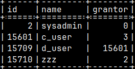
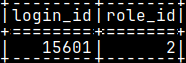
We can see in the sys.auths table that "c_user" created "d_user", because he has "sysadmin" role. The role "zzz" was created by the "sysadmin" role. SELECT * FROM sys.user_role; SELECT * FROM sys.auths WHERE id IN ( 2, 15601, 15709, 15710 );
Grant a Role
We are still "c_user" and we will grant a role to "a_user". GRANT ZZZ TO a_user;
We will fail.
Just like previously, we have to grant a role from a CURRENT_ROLE. GRANT ZZZ TO a_user FROM CURRENT_ROLE;
Now it works.
The "a_user" will be now able to use "ZZZ" role, but he will not be able to grant that role further to the "b_user". I want to change that.
I will revoke "ZZZ" from "a_user". REVOKE ZZZ FROM a_user FROM CURRENT_ROLE;
Then, I will grant him the same role, but with ADMIN rights for that role. GRANT ZZZ TO a_user WITH ADMIN OPTION FROM CURRENT_ROLE;
We'll now jump to be "a_user". mclient -u a_user -d voc #password "1" SET ROLE ZZZ; GRANT ZZZ TO b_user;
This works. Now "b_user" also has "ZZZ" role assigned.
Role Hierarchy
I will create two roles. Then I will create a hierarchy between them.
mclient -u monetdb -d voc
CREATE ROLE ParentRole;
CREATE ROLE ChildRole;
I will now grant "ChildRole" to "ParentRole", with ADMIN OPTION.
GRANT ChildRole TO ParentRole WITH ADMIN OPTION; This is how we create hierarchy. "ParentRole" can delegate "ChildRole".
I will then give some privilege to the ChildRole. Just so we can test it.
GRANT SELECT ON b_user.b_table TO ChildRole;
In the next step, I will grant only the ParentRole to the "c_user".
GRANT ParentRole TO c_user;
We haven't granted ChildRole to the "c_user" but he will still be able to use it by utilizing the hierarchy. mclient -u c_user -d voc #password "1" SET ROLE ParentRole; GRANT ChildRole TO c_user FROM CURRENT_ROLE; SET ROLE ChildRole; SELECT * FROM b_user.b_table;
So, "c_user" will SET the role "ParentRole", and then he will use "WITH ADMIN OPTION" right to delegate "ChildRole" from the "ParentRole" to himself.
After the grant, he can use SET ROLE ChildRole to get access to the table "b_user.b_table".
System Tables
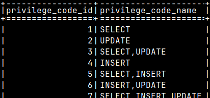
Sistem table "sys.privilege_codes" contains code for all of the possible combinations of SELECT, UPDATE, INSERT, DELETE, TRUNCATE, GRANT.
SELECT * FROM sys.privilege_codes ORDER BY privilege_code_id;
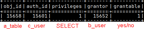
In the table "sys.privileges" we can find the list of the given privileges. On the image we can see that "b_user" gaved "c_user" SELECT grantable rights on the "a_table". SELECT * FROM sys.privileges WHERE obj_id = 15658;
An identity is a symbolic representation of a person, object, or software. It can be a name, a code, or a number. Whenever we read this symbolic representation, we immediately know who/what it is.
Person
Computer
ERP program instance
BI program instance
Aung San
DESKTOP-9A3F2KJ
SAP\36
7892163
From the computer systems perspective, identity is a symbolic representation that can be authenticated and authorized to interact with a system.
Authentication is verifying of the identity.
Person "Aung San" has password "123".
Authorization is a list of things you're allowed to do.
"Aung San" can change and use any object in MonetDB schema "cars_schema".
When we register such identity in some computer system, then we have created an "Account".
For example, library has identity registered as an account.
If we provide our library card, we can be authenticated and then we will be authorized to borrow the book.
User "monetdb"
After the installation of MonetDB, we start with administrator user. His name is "monetdb" and password is "monetdb".
SELECT * FROM sys.auths;
In the system table "sys.auths", we have list of all of the users and roles. Here we can see that ID of the user "monetdb" is number 3.
We can see that this user is admin, because he is the owner of all the system schemas. => SELECT * FROM sys.schemas;
Create a User in MonetDB
We have already seen how to create a user. We need the user's identity ("username") and their authentication ("password"). We will define later what permissions this user has. Only administrators can create new users, so we will login as "monetdb" and we will create new user.
mclient -u monetdb -d voc --password is monetdb CREATE USER "User1" WITH PASSWORD '123' NAME 'Aung San';
"User1" is the username. "Aung San" is the full name of the user.
Auths table has a list of all of the users and roles: SELECT * FROM sys.auths;
We can also find new user in "SELECT * FROM sys.users;".
<= SELECT * FROM sys.schemas; We can also notice that a schema for this new user is created. It has the same name as a user. This is his default schema.
It is not possible to create a user who doesn't have a password.
Preparing a Sample Table
While we are still logged in as administrator, I will create one table. CREATE TABLE schemaTest ( Number INT ); INSERT INTO schemaTest ( Number ) VALUES ( 1 ); SELECT * FROM sys.schemaTest;
GRANT SELECT ON sys.schemaTest TO "User1";
I will also grant the rights to "User1" to be able to read from the table "sys.SchemaTest".
Schemas for the New User
We will quit current session with "quit". Then we will log in as a new user: mclient -u "User1" -d voc --password is 123 SELECT CURRENT_SCHEMA;
If we check the default schema of a user, it will be "User1".
CREATE TABLE schemaTest ( Letter CHAR );
INSERT INTO schemaTest ( Letter ) VALUES ( 'A' );
SELECT * FROM "User1".schemaTest;
We already knew that the new table will be created within the default schema "User1".
I will now alter "User1". ALTER USER "User1" SCHEMA PATH '"sys","User1"';
I will also change the current schema. SET SCHEMA voc;
And then I will read from schemaTest; SELECT * FROM schemaTest;
We will get a table with the "1". That is the table from schema "sys". The reason is that a table is searched for in this order: 1) First search in the current schema. Current schema is "voc" and we will find nothing. 2) Then search in order "sys", "User1" ( SCHEMA PATH attribute ). We will find a table in a "sys" schema and we will return table with the number "1".
CREATE TABLE Test ( Test INT );
If the user "User1" tries now to create a table, MonetDB will try to create a table in the current schema "voc". This will fail because of privilages.
So, unqualified table name is always created in the current schema. Unqualified table in SELECT is searched in schemas in the order "voc" (current schema), "sys" (first schema in the SCHEMA PATH list), "User1" (second schema in the SCHEMA PATH list), and then the other schemas in the SCHEMA PATH list.
Deleting a User
We saw that when we create a user without specifying his schema, a new schema is created.
DROP USER "User1"; –It seems that we can not delete the user because of his schema.
DROP SCHEMA "User1"; — We can not delete schema because it is user's default schema.
ALTER USER "User1" SET SCHEMA sys;
DROP SCHEMA "User1" CASCADE;
DROP USER "User1";
* we have to cascade to delete dependent table "User1".schemaTest.
Solution is that first we change user's default schema. After that we can delete that schema. Then we can delete the user.
Creating a User with Attributes
mclient -u monetdb -d voc
I will quit the session, and then I will login as an administrator. Then I can create another user.
CREATE USER sali WITH PASSWORD '123' NAME 'Sali Noyan'
        SCHEMA sys SCHEMA PATH '"sys","voc"'
        MAX_MEMORY 1073741824 MAX_WORKERS 6
        OPTIMIZER 'minimal_fast';
When creating a new user, we can define many attributes. We can define default schema and schema path. User's query can use maximally 1 GB of memory, and can be processed with 6 CPU threads. Query will use "minimal fast" optimizer.
Default schema
Schema path
Maximal memory for queries
Maximal threads for query
Optimizer used
SCHEMA sys
SCHEMA PATH '"sys","voc"'
MAX_MEMORY 1073741824
MAX_WORKERS 6
OPTIMIZER 'minimal_fast'
We can read from the system table: SELECT * FROM sys.optimizers;
That query will give us a list of the possible optimizers. Optimizers are used to make our queries faster. We should mostly stick with the default optimizer "default_pipe".
Encrypted Password
When we create the user, his password will be encrypted and stored. MonetDB is, by default, using SHA-512 encryption.
If our password is "123" then we can go to the web site https://sha512.online, and there we can encrypt that password into SHA-512 encryption.
Instead of giving MonetDB the task of encrypting password, we can encrypt it ourself. We can, then, create a new user by using that already encrypted password.
If we are administrator, this is how we can create a new user by using encrypted password.
CREATE USER Test WITH ENCRYPTED PASSWORD '3c9909afec25354d551dae21590bb26e38d53f2173b8d3dc3eee4c047e7ab1c1eb8b85103e3be7ba613b31bb5c9c36214dc9f14a42fd7a2fdb84856bca5c44c2' NAME 'Test' SCHEMA sys;
After that, we will quit the session, and then we will log as a new user.
mclient -u test -d voc User will use original password "123". That password will then be encrypted and compared with the stored password.
I will now quit this session and then I will log as an administrator. After that I will delete "test" user.
mclient -u monetdb -d voc--password "monetdb"
DROP USER Test;
Altering Users
We can change the name of a user.
ALTER USER sali RENAME TO merik;
I will change "monetdb" password to "monetdb2" and back. This is for the users to change their own passwords.
ALTER USER SET PASSWORD 'monetdb2' USING OLD PASSWORD 'monetdb'; ALTER USER SET PASSWORD 'monetdb' USING OLD PASSWORD 'monetdb2';
ALTER USER merik
WITH PASSWORD '456'
SET SCHEMA voc
SCHEMA PATH '"sys","voc"'
MAX_MEMORY 1000
MAX_WORKERS 5;
<= This is how admin can change all of the attributes of a user. In this statement each subclause is optional. For example, statement bellow will change only the MAX_MEMORY and MAX_WORKERS. We will turn them of.
ALTER USER merik NO MAX_MEMORY NO MAX_WORKERS;
It seems that is not possible to change OPTIMIZER for a user.
We can now observe changes on the "merik" user.
SELECT * FROM sys.users WHERE name = 'merik';
ALTER with Encrypted Passwords
We can use encrypted version of a password in the ALTER statements.
This can be used by the user: -- ALTER USER SET ENCRYPTED PASSWORD '3c9909afec25354d551dae21590bb26e38d53f2173b8d3dc3eee4c047e7ab1c1eb8b85103e3be7ba613b31bb5c9c36214dc9f14a42fd7a2fdb84856bca5c44c2' USING OLD PASSWORD '456';
This is how admin would change the password of some other user, by using SHA-512. ALTER USER merik WITH ENCRYPTED PASSWORD '3c9909afec25354d551dae21590bb26e38d53f2173b8d3dc3eee4c047e7ab1c1eb8b85103e3be7ba613b31bb5c9c36214dc9f14a42fd7a2fdb84856bca5c44c2';
I will delete the user, "DROP USER merik;".
Roles
Role is a named set of privileges that can be granted to a user. Privileges are permissions to perform an action (e.g., SELECT, INSERT, EXECUTE). Instead of granting individual permissions, we assign a role, and the user inherits all the permissions associated with that role.
In chess, the rights to control each white piece are united under the role of "White".
The rights to control each black piece are united under the role of "Black".
In one match you can accept the role of White, but in another match you can be Black player. Each role can give different rights to the same chess player.
Creation of a New Role
When a new role is created it only has a name. We will see later how to add privileges to a role.
I will create a new user: CREATE USER newUser WITH PASSWORD '123' NAME 'newUser name' SCHEMA sys; New role with the id "15554" will appear in the sys.auths table. This role can not be given to other users; it is the personal property of the "newUser". This personal role will not appear in the sys.roles table.
SELECT *
FROM sys.auths;
SELECT *
FROM sys.roles;
This is how we create the real role. CREATE ROLE newRole; It will appear both in sys.auths and sys.roles.
These kinds of roles can be asign to users.
Default Role
Default role is automatically active for the user upon login and used to determine their default permissions.
In sys.users table we can find data about "newUser" user. SELECT * FROM sys.users WHERE name = 'newuser';
His default role is 15554. That is the personal role created together with that user. SELECT * FROM sys.auths WHERE name = 'newuser';
We can change the default role. I will set "newRole" as a default role for the "newUser".
ALTER USER newUser DEFAULT ROLE newRole;
We can read default role again. Role with ID 15557is "newRole". SELECT name, default_role FROM sys.users WHERE name = 'newuser';
We can assign a default role to a user when the user is created.
CREATE USER mnm WITH PASSWORD '123' NAME 'mnm'
    SCHEMA sys
DEFAULT ROLE newRole; SELECT name, default_role FROM sys.users WHERE name = 'mnm';
Granting a Role
We are currently admin. We can find that out like this: SELECT CURRENT_USER, CURRENT_ROLE;
Admin is using his personal role. This is his default role.
Admin must first grant himself a right to use "newRole". "SET" will not work without that.
SET ROLE newRole;
I want to give admin the right to use newRole. GRANT newRole TO monetdb;
Admin now has the right to use "newRole". We will then make this role the current_role. SET ROLE newRole;
We can now test, what is the current role. SELECT CURRENT_USER, CURRENT_ROLE;
We have successfully changed current role for admin.
Each user, beside the default role, can have several other roles assigned. He can easily switch between them. For example, "SET ROLE monetdb;" will return original admin role to him.
We can find a list of granted roles in the system table: SELECT * FROM sys.user_role; User with ID 3 is admin. User with ID 15581 is "mnm".
When we have created the "mnm", we have set his default role to "newRole" ( 15557 ). That role is then automatically granted to him. We have also ALTER the user "newUser". We gave him default role "newRole" ( 15557 ), but in that case this role was not granted to him automatically. This is not good. If we alter the user default role, that role should be automatically granted to him. It is wrong that user, after he log in, have a default role that he was not granted. We can solve this problem by granting the role separately.
GRANT newRole TO newUser;
SELECT * FROM sys.user_role;
Deleting a Role
We can easily delete the role. DROP ROLE newRole; SELECT * FROM sys.roles;
CREATE TABLE trigTab ( Number INT );
CREATE TABLE logTab ( Pre INT, Post INT );
SELECT * FROM trigTab; SELECT * FROM logTab;
The task is that for each change in "trigTab", we remember the change in the "logTab". These are the changes in the "trigTab":
1) INSERT INTO trigTab VALUES ( 1 );

2) UPDATE trigTab SET Number = 2 WHERE Number = 1;

3) DELETE FROM trigTab WHERE Number = 2;
Each time we change something in "trigTab", we will remember that change in the "logTab".
1) INSERT INTO logTab VALUES ( null, 1 );

2) INSERT INTO logTab VALUES ( 1, 2 );

3) INSERT INTO logTab VALUES ( 2, null );
Although now, our "trigTab" is empty, we have "logTab" with the whole history of changes in the "trigTab".
We want to automate remembering this history and for that we can use triggers.
Triggers
A SQL trigger is a database object that automatically executes a predefined set of SQL statements in response to certain events occurring on a specific table. In our example, each DML statement on a "trigTab" will trigger the change on the "logTab". Like a knee-jerk reaction.
A trigger is defined on a table. When we delete that table, the associated trigger will also be deleted. The response of a trigger is an SQL procedure. Any set of statements that we can put into a procedure can be used as the response of a trigger.
This is an example of a trigger that will be triggered each time we insert some number into "trigTab".
CREATE OR REPLACE TRIGGER trigINSERT --create a new trigger AFTER INSERT ON trigTab --this trigger is activated after each insert into trigTab REFERENCING NEW ROW AS NewRow--we can reference inserted values as RecordAlias.ColumnName FOR EACH ROW --this trigger will be activated once for each inserted number BEGIN ATOMIC --this is trigger response: INSERT INTO logTab VALUES ( null, NewRow.Number ); --we insert null and new value into logTab END;
We will insert 2 numbers into trigTab and that will start a knee-jerk reaction. INSERT INTO trigTab VALUES ( 1 ), ( 2 );
Message is saying that 4 rows will be affected. Two are in the "trigTab", and two are the response in the "logTab". SELECT * FROM trigTab; SELECT * FROM logTab;
Triggers Theory
Triggers are used to automate some actions. We are using triggers when we want to:
Enforce business rules and formatting of data.
Enforce integrity rules. Changes to multiple tables should occur simultaneously.
In denormalized schemas, we can use triggers to update summary tables.
When we want to log the changes made.
Triggers are powerful, but big power can create big problems:
Triggers are reducing server performance and they increase database locking.
Triggers are hard for debugging.
Triggers create dependency between database objects. This makes modifying of a database harder.
We can easily forget that triggers exist and can be confused by unexpected changes in our data.
It is difficult to determine in what order the triggers will be activated (if we have several triggers of the same type on one table).
When using triggers we should follow next rules:
Limit the number of triggers of the same type on one table.
Don't place complex logic into triggers.
Avoid cascading triggers. Cascading trigger is a trigger that can activate some other trigger. This can lead to hard-to-debug behavior or infinite loops.
Always document triggers. Document why the trigger do exist, what does it work, are there any exceptions or caveats to how the trigger works.
Triggers can not be activated directly, only indirectly. Triggers can not accept arguments.
BEFORE and AFTER
Some change on a table will activate the trigger. Our response to that change can be done before or after the change. We can be proactive or reactive.
CREATE OR REPLACE TRIGGER trigTRUNCATE BEFORE INSERT ON trigTab --this trigger is activated before each insert into trigTab REFERENCING NEW ROW AS NewRow FOR EACH ROW --this trigger will be activated once for each row WHEN ( NewRow.Number IN ( 0, 1 ) )--only when we try to insert zero or one BEGIN ATOMIC DELETE FROM trigTab; --before inserting the 0 or 1, we'll empty trigTab END;
This trigger will be proactive. We will act BEFORE the INSERT event.
Before we insert a zero, or one in the table "trigTab", we will empty the same table.
Let's initiate our trigger. Again, we will insert two values. Before the insert, I will empty "trigTab" table. TRUNCATE trigTab; INSERT INTO trigTab ( Number ) VALUES ( 0 ), ( 1 );
We can now read from the table "trigTab"; SELECT * FROM trigTab;
Suprisingly, we'll have two numbers in our table. This is because BEFORE trigger will fire twice, before the INSERT even started. So, "trigTab" will be deleted twice, and then the two numbers will be inserted.
This is not the consequence of the transaction isolation. Inside one transaction we can insert one value in a table and then read it. This is the consequence of the fact that all of the BEFORE responses will be executed before the changes in a table are made.
Let's test this with AFTER trigger. I will first clear the environment.
TRUNCATE trigTab;
TRUNCATE logTab;
DROP TRIGGER trigTRUNCATE;
DROP TRIGGER trigINSERT;
CREATE OR REPLACE TRIGGER trigCOUNT
AFTER INSERT ON trigTab
REFERENCING NEW ROW AS NewRow
FOR EACH ROW
WHEN ( NewRow.Number IN ( 0, 1 ) )
         BEGIN ATOMIC
                  DECLARE NumberOfRows INT;
                  SET NumberOfRows = ( SELECT COUNT( * ) FROM trigTab );
                  INSERT INTO logTab ( Pre, Post ) VALUES (NewRow.Number, NumberOfRows);
         END;
After each insert into "trigTab" table, we will register how many rows this table has. We will use the table "logTab" to remember these results.
We will now test AFTER trigger. INSERT INTO trigTab ( Number ) VALUES ( 0 ), ( 1 ); We will then read from the "logTab". I will change the names of columns of this table to appropriate aliases.
SELECT pre AS InsertedValue, post AS NumberOfRows
FROM logTab;
We can see that "NumberOfRows" is always 2. That means that we have first executed INSERT statement, and only then did we execute AFTER triggers.
"SELECT COUNT( * ) FROM trigTab" will be run twice, but only after the INSERT INTO has finished.
Can We Intercept and Modify the Change on a Table?
In MonetDB, triggers are either proactive (BEFORE) or reactive (AFTER), so they can not modify the statement that activates them. Let's assume that when a user wants to insert number X into "trigTab", our trigger should intercept that statement and modify number X into ( X +1 ), so that ( X + 1 ) is going to be inserted instead. This is not possible to do in the MonetDB, but we can get the same result by altering the value X in the table into ( X + 1 ), by the AFTER trigger.
I will clear the environment:
TRUNCATE trigTab;
TRUNCATE logTab;
DROP TRIGGER trigCOUNT;
CREATE OR REPLACE TRIGGER trigINTERCEPT
AFTER INSERT ON trigTab
REFERENCING NEW ROW AS NewRow
      FOR EACH ROW
BEGIN ATOMIC UPDATE trigTab SET Number = NewRow.Number + 1 WHERE trigTab.Number = NewRow.Number; END;
This trigger will use UPDATE to transform X into ( X + 1). Note that we have to use prefix "trigTab" when defining WHERE condition.
We'll induce the change, and then we will read from the "trigTab". INSERT INTO trigTab ( Number ) VALUES ( 19 ); SELECT * FROM trigTab; We can see on the image that number 19 is increased by 1, so we have number 20.
In this solution it is necessary that we have a way to identify a row that was changed, so that we can overwrite the original change. The example bellow will better explain this problem.
INSERT INTO trigTab ( Number ) VALUES ( 20 );
SELECT * FROM trigTab;
We inserted number 20 into table that already has number 20. This time the trigger will not know what row to change, so it will change both of them, so that is why we have 21 twice. Such trigger can be useful only if we can uniquely identify the changed row.
Triggers Activated by DELETE and TRUNCATE
I will clear the environment:
DROP TRIGGER trigINTERCEPT;
CREATE OR REPLACE TRIGGER trigDELETE AFTER DELETE ON trigTab REFERENCING OLD OldRow FOR EACH ROW BEGIN ATOMIC INSERT INTO logTAB ( pre, post ) VALUES ( OldRow.Number, null ) ; END;
DELETE FROM trigTab; After delete, we can only reference old rows. SELECT * FROM logTab;
Everything will work the same for the TRUNCATE.
Triggers Activated by UPDATE
I will prepare the environment:
INSERT INTO trigTab VALUES ( 5 );
TRUNCATE logTab;
DROP TRIGGER trigDELETE;
CREATE OR REPLACE TRIGGER trigUPDATE BEFORE UPDATE ON trigTab REFERENCING OLD OldRowNEW NewRow--no comma between FOR EACH ROW BEGIN ATOMIC INSERT INTO logTAB ( pre, post ) VALUES ( OldRow.Number, NewRow.Number ); END;
UPDATE trigTab
SET Number = 6 WHERE Number = 5;
With UPDATE, we can reference both old and new values. SELECT * FROM logTab;
We can limit UPDATE trigger only to changes in some of the columns. I will prepare the environment once more:
TRUNCATE trigTab;
DROP TRIGGER trigUPDATE;
CREATE OR REPLACE TRIGGER trigUpdateOf
BEFORE UPDATE OF pre ON logTab
REFERENCING OLD OldRow NEW NewRow
       FOR EACH ROW
       BEGIN ATOMIC
              INSERT INTO trigTab VALUES ( OldRow.Pre * 10 + NewRow.Pre );
       END;
This trigger will be activated only if someone update a value in the "pre" column. This time I have reversed the roles of the "trigTab" and "logTab" tables. Changes on "logTab" will be logged into "trigTab".
UPDATE logTab SET post = 7 WHERE post = 6;
SELECT * FROM trigTab;
Update statement is changing only the column "post". That means that this trigger should not be activate. We can see on the image that the trigger was activated. We can conclude that "UPDATE of" doesn't work in MonetDB.
CREATE OR REPLACE TRIGGER trigUpdateOf
BEFORE UPDATE OF pre ON logTab
REFERENCING OLD OldRow NEW NewRow FOR EACH ROW WHEN ( OldRow.Pre <> NewRow.Pre ) BEGIN ATOMIC INSERT INTO trigTab VALUES ( OldRow.Pre * 10 + NewRow.Pre ); END;
Maybe this will work instead of "UPDATE of"? But it wont. It seems that we can not use OldRow.Pre in the WHENsubclause. We can only use NewRow.Pre.
CREATE OR REPLACE TRIGGER trigUpdateOf
BEFORE UPDATE OF pre ON logTab
REFERENCING OLD OldRow NEW NewRow
       FOR EACH ROW
       BEGIN ATOMIC
             IF ( OldRow.Pre <> NewRow.Pre ) THEN
                     INSERT INTO trigTab VALUES ( OldRow.Pre * 10 + NewRow.Pre );
             END IF;
       END;
This version is using IF statement to control flow. This trigger will be accepted by MonetDB, but when we try to update something: UPDATE logTab SET pre = 99; , we will get an error.
It seems to me that currently we can not compare old and new values in MonetDB UPDATE trigger.
FOR EACH STATEMENT
I will clear the environment:
TRUNCATE trigTab;
TRUNCATE logTab;
DROP TRIGGER trigUpdateOf;
Triggers don't have to be activated for each row that is changed. Triggers can be activated only once for the whole statement.
CREATE OR REPLACE TRIGGER trigStatement
BEFORE INSERT ON trigTab
REFERENCING NEW TABLE AS NewTable
       FOR EACH STATEMENT
       BEGIN ATOMIC
              DECLARE NoOfRows INTEGER;
              SET NoOfRows = ( SELECT COUNT(*) FROM newTable );
              INSERT INTO logTab VALUES ( NoOfRows, null );
       END;
Instead of "FOR EACH ROW", we now have "FOR EACH STATEMENT". Instead of "NEW ROW", we now have "NEW TABLE".
"NewTable" represents all of the inserted rows (only the changed rows). We can use COUNT(*) to find the number of inserted rows.
INSERT INTO trigTab VALUES ( 13 ), ( 17 );
SELECT Pre AS "NoOfRows" FROM logTab;
I am using alias "NoOfRows" to correctly label the column.
After inserting 2 values, "logTab" table now has 2 rows.
When using UPDATE trigger, we can also use variable "OLD TABLE". "NEW TABLE" represents changed rows, and "OLD TABLE" represents those rows before the change.
Statement Instead of the Procedure
If our trigger has to only execute one statement as response, we don't have to use syntax for a procedure. We can just write that one statement.
I will clear the environment:
TRUNCATE trigTab;
TRUNCATE logTab;
DROP TRIGGER trigStatement;
CREATE OR REPLACE TRIGGER trigNoProcedure AFTER INSERT ON trigTab FOR EACH ROW INSERT INTO logTAB VALUES ( 88, 88);
We don't need syntax BEGIN ATOMIC and END if we only have one statement.
INSERT INTO trigTab VALUES ( 1 );
SELECT * FROM logTab;
Special Triggers
Triggers on Views
Because MonetDB views are not updateable, it is not possible to create triggers on views.
LOGIN Triggers
LOGIN triggers can be activated before or after the user have login to MonetDB server.
CREATE OR REPLACE TRIGGER trigSchema
AFTER LOGIN
       BEGIN ATOMIC
              SET SCHEMA voc;
       END;
We can use a trigger like this to change a user's default schema after they log in. It seems that these LOGIN triggers don't work. I have tried several variants of such triggers and I have never succeeded to make them working.
Recursive Triggers
I will clear the environment.
TRUNCATE trigTab;
TRUNCATE logTAB;
DROP TRIGGER trigNoProcedure;
Each trigger is doing some action in a response to triggering event. In the example below we can see trigger that will response with an INSERT statement, but that INSERT statement will call the same trigger again. In that way we have an endless loop. MonetDB will response with the error message.
CREATE OR REPLACE TRIGGER trigRecursive
BEFORE INSERT ON trigTab
FOR EACH ROW
     INSERT INTO trigTab VALUES ( 21 );
INSERT INTO trigTab VALUES ( 14 );
I will now delete trigRecursive with "DROP TRIGGER trigRecursive;".
We can also have two triggers that are mutually recursive.
CREATE OR REPLACE TRIGGER trigBefore
BEFORE TRUNCATE ON logTab
FOR EACH ROW
     INSERT INTO trigTab VALUES ( 21 );
CREATE OR REPLACE TRIGGER trigAfter
AFTER INSERT ON trigTab
FOR EACH STATEMENT
     TRUNCATE logTab;
TRUNCATE logTAB;
"trigBefore" is doing INSERT, which will start "trigAfter". "trigAfter" is doing TRUNCATE, which will call "trigBefore". This is vicious cycle that will never end and MonetDB will response with the error message. We should strive to avoid such situations.
System Table
Data about our triggers can be found in sys.triggers system table.


 Admin is using his personal role. This is his default role.
 We have successfully changed current role for admin.


 After inserting 2 values, "


