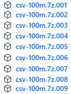
For this benchmark we will use sales data from the fictitious company "Contoso". We can download our database from the github. If we go to this address, we will find there compressed CSV files with the data. In total there are 8 files of 500 MB, and one smaller file with 250 MB ( 4250 MB in total ).
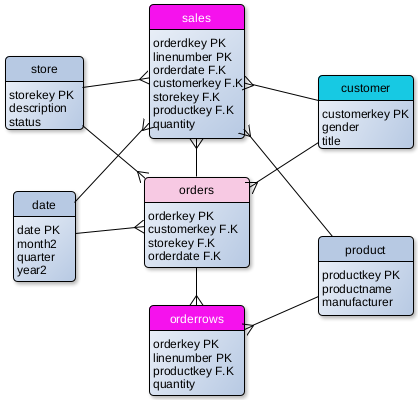
When we unzip these files, inside we will find 8 CSV files. This is sales cube with tables that can show us sales and orders per product, customer, date and store.
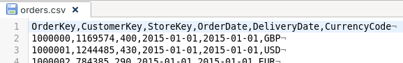
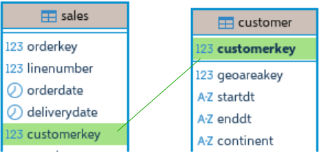
Three big tables are "Orders" ( 88M ), "Sales" ( 211M ) and "OrderRows" ( 211M ). Dimension table "Customer" has 2M rows, and all the other dimension tables are small.
Not all of the columns are shown on the image.
—————————————————————————————— In CSV file "date.csv" I will change the names of columns month=>month2 and year=>year2, because MonetDB will not accept original names. "Month" and "Year" are reserved words.
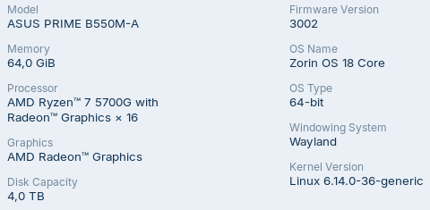
Machine Hardware
For this benchmark we will use CPU with 8 cores and 64 GB of RAM.
Our operational system is Zorin 18.
Creating Tables and Loading CSV Files
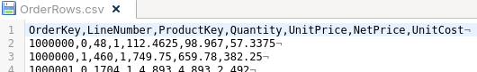
OrderRows Table
CREATE TABLE orderrows (
OrderKey BIGINT NOT NULL,
LineNumber SMALLINT NOT NULL,
ProductKey SMALLINT NOT NULL,
Quantity SMALLINT NOT NULL,
UnitPrice REAL NOT NULL, --DECIMAL(8,4)
NetPrice REAL NOT NULL, --DECIMAL(10,6) UnitCost REAL NOT NULL --DECIMAL(8,4) );
First, I will create table for OrderRows in the MonetDB. I will not create primary and foreign key constraints this time.
I will fill this table from my CSV file with "COPY INTO" statement.
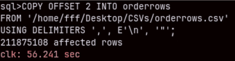
COPY OFFSET 2 INTO orderrows
FROM '/home/fff/Desktop/CSVs/orderrows.csv'
USING DELIMITERS ',', E'\n', '"'
NULL AS '';
Import of this 211M rows table will last only one minute ( 56.241 sec ). Amazing.
Other Tables
I will leave a file for download at the end of this article. That file will have SQL for creation and import of all of the Contoso tables.
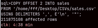
Bellow we can see time for import for two other larger files. Smaller dimension tables are imported almost instantly.
Sales (211M) table will need almost 5 minutes to be imported.
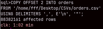
Orders (88M) CSV table will be imported in 62 seconds.
Query Benchmarking
Cold Start
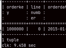
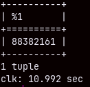
I will now restart my computer. I want to make sure to run a cold query. This simple query bellow will run for 10 seconds. MonetDB database becomes faster as more queries are executed. This ability of MonetDB is called "cracking". MonetDB will automatically sort, group and index columns during the SELECT queries. That will make subsequent queries faster.
SELECT * FROM sales LIMIT 1;
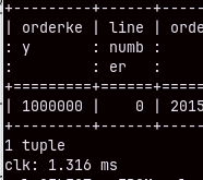
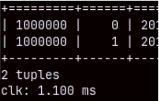
If we run this query again, it will be executed in just 1.3 miliseconds. This is not the result of query caching. If we make a query that takes 2 or 3 rows, we will again see these exceptional speeds.
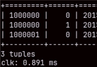
SELECT * FROM sales LIMIT 2; SELECT * FROM sales LIMIT 3;
Aggregated Queries in MonetDB
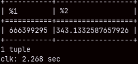
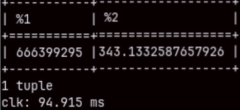
If we aggregate two columns in the "sales" table, that query will touch 211M rows. It will be fast ( 2.268 sec. ), but we can repeat it to get only 94.915 ms.
SELECT SUM( quantity ), AVG( unitprice ) FROM sales;
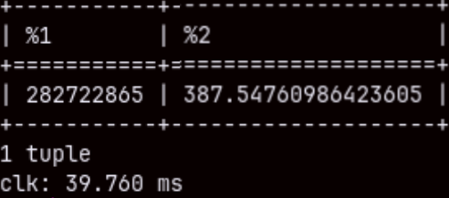
I will run the same query, but this time with a filter. SELECT SUM( quantity ), AVG( unitprice ) FROM sales WHERE orderdate <= '2020-05-25';
We will get the result even faster. This proves that the result is not cached. MonetDB run the query again, but this time "cracking" made our query faster.
It's hard to make a benchmark when execution times are constantly changing. So, from now on I will focus on the fastest times.
How Database Reports Execution Time
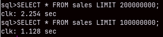
SELECT * FROM sales LIMIT 1000000;--13 ms SELECT * FROM sales LIMIT 2000000; --24 ms
MonetDB is reporting that the second query is slower than the first one. That is something that we are expecting. The problem is that according to my computer clock the first query was finished after 7 seconds, and the second one after 15 seconds.
Databases only report the time spent to produce the results in the memory. It will not include the time needed to print the result in the shell or any other client. That is why MonetDB is reporting 13 ms, but I can see the result only after 7 seconds. MonetDB has command to suppress printing of the result in the shell. I will use that command ( command explained here ) next, to test reading the whole tables.
This is how long it takes MonetDB to read a large number of rows. Columnar databases are better suited for aggregate queries, but we can see that MonetDB is capable of performing OLTP types of queries quite well.
I will disable my command, so we can again see the results of our queries.
Joins
SELECT productkey, SUM( quantity ), AVG( netprice ) FROM sales GROUP BY productkey;
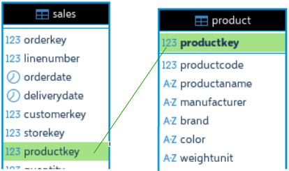
This query will execute for 340 ms. If we want to see brands then we have to make a join between "product" and "sales" tables.
SELECT brand, SUM( quantity ), AVG( netprice ) FROM sales INNER JOIN product ON sales.productkey = product.productkey GROUP BY brand;
The query with a join will last more than 1 second. We can speed it up if we create a foreign key constraint.
Now that we have foreign key constraint, the query from before will become 200 ms faster. That is 20% faster.
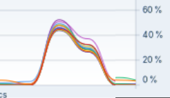
Query from before is a traditional analytical query. If we look at system monitor, we will see that during the execution of this query the load will be equally distributed between CPU cores. MonetDB is capable to significantly parallelize query execution. That means that our individual queries can be speed up with a CPU that has even more cores.
DISTINCT, LIKE, ROLLUP
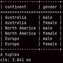
From the table "customer" we can list distinct continents and genders in 3.841 ms.
SELECT DISTINCT continent, gender FROM customer;
We can get distinct combinations of storekey and currency code from "sales" table in half of the second.
SELECT DISTINCT storekey, currencycode FROM sales;
If we want to count unique combinations of the orderkey and currencycode, then our query will be slow, it will last almost 11 seconds. But this query has to count 88 million rows.
SELECT COUNT( * ) FROM
     ( SELECT DISTINCT orderkey, currencycode
       FROM sales );
Query like this will also last 11 seconds.
SELECT COUNT( * ) FROM
  ( SELECT orderkey, currencycode
     FROM sales
     GROUP BY orderkey, currencycode );
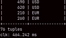
LIKE operator allows usage of the wild cards. Sign "_" will replace one letter.
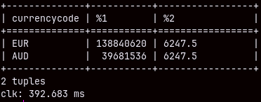
SELECT currencycode, SUM( quantity ), MAX( unitprice )
FROM sales
WHERE currencycode LIKE '_U_' GROUP BY currencycode;
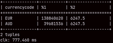
If we use the sign "%" that replaces several characters, then the speed will drop, almost double.
SELECT currencycode, SUM( quantity ), MAX( unitprice )
FROM sales
WHERE currencycode LIKE '%U_' GROUP BY currencycode;
Before we test ROLLUP, I will create foreign key constraint between "customer" and "sales" tables.
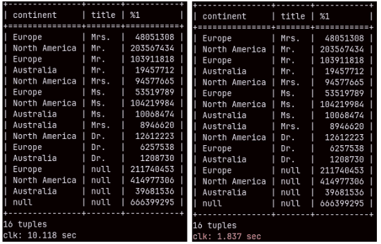
This time we have unusually slow query. It will take full 10 seconds. SELECT continent, title, SUM( quantity ) FROM customer INNER JOIN sales ON customer.customerkey = sales.customerkey GROUP BY ROLLUP( continent, title ); ——————————————————————————————————————————– Query with union would be much better choice for this. Only 1.837 seconds. SELECT continent, title, SUM( quantity ) FROM sales INNER JOIN customer ON sales.customerkey = customer.customerkey GROUP BY continent, title UNION SELECT continent, null, SUM( quantity ) FROM sales INNER JOIN customer ON sales.customerkey = customer.customerkey GROUP BY continent UNION SELECT null, null, SUM( quantity ) FROM sales;
This show us that there is still room for improvements in MonetDB optimizer.
Window Functions
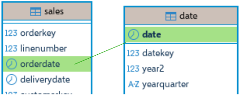
I will first add foreign key constraint between "sales" and "date" tables.
ALTER TABLE date ADD CONSTRAINT date_pk PRIMARY KEY ( date );
ALTER TABLE sales ADD CONSTRAINT FKfromDate FOREIGN KEY ( orderdate ) REFERENCES date ( date );
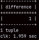
We can use LAG function to compare sales for the current and the previous row. Each value from quantity column will have a pair in the BeforeQty column, except in the first row ( no previous ). Quantity in that first row will make a difference. This query will execute in 2 seconds.
SELECT ( SUM( Qty ) - SUM( BeforeQty ) ) AS Difference FROM
( SELECT Quantity AS Qty,
  LAG( Quantity, -1 ) OVER ( ORDER BY date ) AS BeforeQty
  FROM date INNER JOIN sales ON date.date = sales.orderdate );
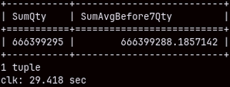
For each row in the table, we will calculate the average quantity of the previous 6 rows and the current row. At the end will see sums of the quantity and these rolling averages. This query will last 29 seconds.
SELECT SUM( Quantity ) AS "SumQty", SUM( AvgBefore7Qty ) AS "SumAvgBefore7Qty" FROM
( SELECT Date, Quantity,
     AVG( Quantity ) OVER
         ( ORDER BY Date ROWS BETWEEN 6 PRECEDING AND CURRENT ROW)
             AS AvgBefore7Qty
FROM date INNER JOIN sales ON date.date = sales.orderdate );
Updates
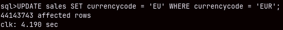
MonetDB should be slow for updates, but it managed to update 44 milion rows for just 4.19 seconds. UPDATE sales SET currencycode = 'EU' WHERE currencycode = 'EUR';
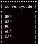
We can confirm that all of the values 'EUR' are updated to 'EU'.
SELECT DISTINCT currencycode FROM sales;
Problematic Queries
Double Grouping
Double grouping is when we first group our data, and then we group that result. For example, we will total sales quantity per customerkey, and then we will count customers per total quantity. We will count how many customers have the same total quantity.
This query is problematic because while the first grouping can be fast, the second one could be much longer. The result of the first grouping will have 2M rows, because we have so much customers. In the second stage, we have to group these 2M rows, and that is when I expect the performance to become bad.
SELECT customer.customerkey, SUM( quantity ) AS TotQty
FROM customer INNER JOIN sales ON customer.customerkey = sales.customerkey
GROUP BY customer.customerkey;
In the first phase I will measure how much time is needed to group by customer. It is 5 seconds because there are 2 million customers.
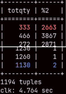
Second phase: SELECT TotQty, COUNT( customerkey ) FROM ( SELECT customer.customerkey, SUM( quantity ) AS TotQty FROM customer INNER JOIN sales ON customer.customerkey = sales.customerkey GROUP BY customer.customerkey ) as FirstPhase GROUP BY TotQty;
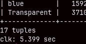
We can see on the image that we have 2,663 customers with total quantity of 333 items, and only two with 1,130 items. The time for execution is again 5 seconds. This is something I didn't expect. I am pleasantly surprised. I can tell you that these kinds of queries are problematic for Power BI database ( SSAS ).
Aggregated Query from Two Fact Tables ( Stitch Query )
This time I will create foreign key constraint on the "OrderRows" (211M) table. I want to aggregate sales and orderrows per product brend. ALTER TABLE orderrows ADD CONSTRAINT FK_Product FOREIGN KEY ( productkey ) REFERENCES product ( productkey );
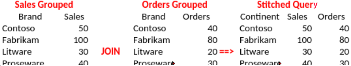
"Stitch" query is when we aggregate two fact tables per the same dimension and we get two data sets as a result. Then we join those two data sets in the final result. This is how we aggregate values from two fact tables.
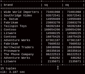
Query bellow will last 7.5 seconds. This is longer than I expected. If we ran subqueries separately the time would be just 900 ms each. Because we only have 15 brands, it is surprising that it will take 5 seconds just to join two small tables. SELECT S.brand, Sq, Oq FROM ( SELECT Brand, SUM( quantity ) Sq FROM Product INNER JOIN Sales ON Product.Productkey = Sales.ProductKey GROUP BY Brand ) S INNER JOIN ( SELECT Brand, SUM( quantity ) Oq FROM Product INNER JOIN Orderrows ON Product.Productkey = OrderRows.ProductKey GROUP BY Brand ) O ON S.Brand = O.Brand;
If we "UNION ALL" our subqueries, the execution will last 7.5 seconds, too. SELECT Brand, SUM( quantity ) Sq FROM Product INNER JOIN Sales ON Product.Productkey = Sales.ProductKey GROUP BY Brand UNION ALL SELECT Brand, SUM( quantity ) Oq FROM Product INNER JOIN Orderrows ON Product.Productkey = OrderRows.ProductKey GROUP BY Brand;
I have tried to read two small subqueries into python, and then to join them with pandas. Python reported execution time of just 1.2 seconds. It is strange that we can get the final result faster by combining MonetDB and Pandas, then just by using MonetDB.
WITH S AS
( SELECT productkey, SUM( quantity ) AS Sq FROM Sales GROUP BY productkey ),
O AS ( SELECT productkey, SUM( quantity ) AS Oq FROM Orderrows GROUP BY productkey ), PS AS ( SELECT brand, SUM( Sq ) AS SQty FROM Product INNER JOIN S ON Product.productkey = S.productkey GROUP BY brand ), PO AS ( SELECT brand, SUM( Oq ) AS OQty FROM Product INNER JOIN O ON Product.productkey = O.productkey GROUP BY brand ) SELECT PS.brand, Sqty, OQty FROM PS INNER JOIN PO ON PS.brand = PO.brand;
We can reduce our fact tables by grouping them by productkey and then following the same logic. This approach would speed up our query to 5.5 seconds.
WITH S AS ( SELECT productkey, SUM(quantity) AS Sq
            FROM sales
            GROUP BY productkey ),
O AS ( SELECT productkey, SUM(quantlty) AS Oq
       FROM orderrows
       GROUP BY productkey )
SELECT P.brand, SUM(S.Sq) AS Sq, SUM(O.Oq) AS Oq
FROM product P
 LEFT JOIN S ON S.productkey = P.productkey
 LEFT JOIN O ON O.productkey = P.productkey
GROUP BY P.brand;
This would be the fastest version of this query. It would execute in only 3 seconds.
In this query, we would use the the last subquery to join reduced sales and orderRows tables, with the product table.
INSERT INTO SELECT
I will use "INSERT INTO SELECT" to make "Sales" table bigger. Before doing that, I will remove FK constraints. I will also change optimizer. ALTER TABLE sales DROP CONSTRAINT fkfromproduct; ALTER TABLE sales DROP CONSTRAINT fkfromcustomer; ALTER TABLE sales DROP CONSTRAINT fkfromdate; SET sys.optimizer = 'minimal_pipe';
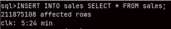
I will now run this statement to make my sales table twice bigger. INSERT INTO sales SELECT * FROM sales; MonetDB needed 5 minutes to do this.
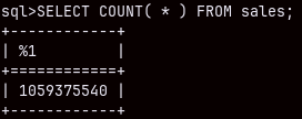
I will do this 1 more time. That will double the number of rows to 844M. That was done in 9:48 minutes. Then, I will again read from the CSV file into this table. That will add another 211M rows, so in total "sales" table will now have one billion rows.
I will recreate foreign key constraint toward "product" table. ALTER TABLE sales ADD CONSTRAINT FKfromProduct FOREIGN KEY ( productkey ) REFERENCES product ( productkey );
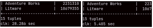
I will run now this query twice. The first time it will end after 28 seconds, and the second time after 5,5 seconds. SELECT brand, SUM( quantity ), AVG( netprice ) FROM sales INNER JOIN product ON sales.productkey = product.productkey GROUP BY brand;
SELECT color, SUM( quantity ), AVG( netprice ) FROM product INNER JOIN sales
    ON sales.productkey = product.productkey
GROUP BY color;
Immediately after, I run the same query, by it was grouped by color. The time was again 5 seconds.
We can see that performance is good, even with 1B rows.
Conclusions
We can conclude some things: – MonetDB is usually very fast. – Initially, until the database worm up, queries can be slow. – We should always set foreign key constraints to achieve speed boost. – Some kinds of queries are better optimized than others.
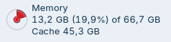
– MonetDB does not use much memory. During the import of the "sales" table, the RAM usage increased from 4 to 13 GB. It was the same during this last, 1B rows, query. At other times, the usage was much less.
Stores like to sell products as a bundle. For example, the store will sell a box with several decorations as one product. Store will benefit from this because: – Stacking and scanning products is easier when the are bundled ( effort- ). – The buyer will spent less time in the store choosing decorations ( speed+ ). – We can sell more decorations by bundling less popular decorations with the more popular ones ( sale+ ).
But bundles make production planning harder. – We have to unbundle data about products to find out how much each individual shape/color was sold ( effort+ ). – We are usually looking at sale for a longer period of time. Because of quantity of data, unbundling will make our database real slow ( speed- ). – We have to read data about all the shapes/colors, although we just want to analyze the sale of one of the shapes/colors ( analysis- ).
Data in Bundle or in Bulk
We can treat transactions as one bundle product. Product code, quantity and price are one bundle. We want to be able to quickly save this data bundle.
We can achieve this by saving our transactions as separate rows in a database. That is how we can quickly save or retrieve individual transaction as a bundle.
For production planning we will differently organize our data. We will organize it into columns. If we want to find out how many products, we have sold that have the price lower than 3 EUR, we just have to scan the column "Price", and then to find specific positions in the column "Qty".
Each column can be sorted and compressed for even faster retrieval.
We don't even need to read the column "Product".
When we organize data in rows, we use a row-oriented database. When we organize data in columns, we use a columnar database. Data is typically collected in a row-oriented database (Postgres, Oracle, MySQL) and then transferred to a columnar database for analytics ( ClickHouse, DuckDB, Vertica ).
Row Oriented Databases vs Columnar Databases
Row oriented databases: 1) They are great for small writes/reads. Perfect for "insert one order", "update this user", "delete this invoice line" etc. 2) Application code often works with whole objects/rows (User, Order, Invoice), which matches row layout. 3) Great for transaction isolation, replication, ACID complacence, constraints, triggers, foreign keys. 4) We have many users who send queries that touch only one row from a table and expect an immediate response from the database.
They are best for Cash registers, ERP, CRM, banking systems, ticketing.
Columnar databases: 1) We only read columns we need, and columns can be heavily compressed. That improves IO. 2) CPU can process several values of the same type at once. This is called vectorized execution. Queries with lot of data will work faster. 3) Column scans and aggregations are easy to parallelize across cores and nodes. 4) We have smaller number of queries, but they are much heavier, they touch a lot of data, with lot of joins, but the users are expecting results in 3-4 seconds.
They are best for sales reports, dashboards, time-series, data mining.
Row oriented databases are catching current state and providing transactional correctness. Columnar databases are for analysis of the historical data. We can also say that row-oriented databases are better in writing data and providing data consistency and integrity. Columnar databases are better in reading huge quantities of data.
OLTP vs OLAP
If we are preparing our database for everyday operations and transactions, then we are making OLTP database. For analytics and BI, we would prepare OLAP database. OLTP is compatible with row-oriented databases, and OLAP with columnar databases.
In the OLTP databases, data is organized in a lot of small tables. There is no data duplication and every value is written only once.
Small tables make queries more complex so these databases usually don't grow significantly in size.
In the OLAP databases, we merge small tables to reduce their number. Columnar technology have no problem with tall tables that have a lot of columns.
By reducing the number of joins, we can query our data with simpler (faster) queries. That is why we organize our tables in a star schema.
OLTP tables are filled with data by users and applications in small transactions. From time to time ( usually nightly ), data is transformed and transported into OLAP databases in batches. This makes data management different between OLTP and OLAP databases. OLTP databases receive data continuously, but OLAP databases receive data periodically and only after data is well-reformed.
OLTP is acronym for "Online Transaction Processing" and OLAP for "Online Analytical Processing". We saw that the difference is made by: – Different purpose and usage. – Different database technology. – Different data organization inside the database. – Different data management.
Data Immutability
Columnar ( OLAP ) databases are filled in batches. That doesn't mean that it is not possible to UPDATE or DELETE rows in tables. There are four strategies that OLAP databases use:
1) Data is immutable. We can only insert data in batches, and afterward we can not change individual rows. If data is immutable and presorted then we can achieve the biggest levels of compression. The example of this technology is the database used for Power BI.
2) MonetDB is an example of the OLAP database that is suited for light updates and deletes. When we delete/update some value, MonetDB will label old record as "dead". That record will become invisible to queries. After some time, garbage collection will remove not-needed records.
3) We can divide our columns into small segments. Whenever we want to change some value, we modify the whole segment. This is good solution when we have a lot of hardware power, like cloud providers do. Google Snowflake is an example of such database.
4) We can have two databases in one. One database is row-oriented, and the other one is columnar. Data is written into row-oriented database, but when we want to read data we read from both databases together. Historical data is read from the columnar database, and today's data is read from the row-oriented database. SAP Hana is using such approach.
This last strategy creates something called "Hybrid Transaction Analytical Processing", or HTAP. HTAP is when a single database can do fast real-time transactions and fast analytics on the same data at the same time.
In recent years, MonetDB researchers have been gradually adding or experimenting with features that move it slightly toward the HTAP category:
– Better handling of frequent updates and small transactions – Improved concurrency and snapshot isolation – Faster incremental data loads – Optimizations for mixed workloads
MonetDB
If you have one server and install MonetDB on it, you will be able to: – Enjoy blazing-fast query performance, even if you have a lot of data and your queries are more complex. – Avoid thinking about indexing, compression, statistics tuning, partitioning decisions. MonetDB will do it all automatically. – Apply the full power of SQL to all your tables, whether they are carefully modeled or just collected in one place. – Spend your money on something else because MonetDB is an open source database under the Mozilla Public License.
MonetDB is a fast, complete SQL, easy-to-maintain, open source analytical database server that can process huge amounts of data on a single server machine.
Hardware and Speed Considerations for MonetDB
MonetDB doesn't have a requirement to keep the whole database in a RAM memory. Parts of data that are already processed will be deleted from memory. MonetDB have capacity to deal with data that is much bigger than the amount of memory on your server machine. Only data that is currently processed will have just-in-memory execution pipelines.
MonetDB, will benefit from the fast NVMe disk, that has sustained performance under write load. Such disk should be accompanied with a lot of RAM memory, so that usage of a disk is minimal.
MonetDB is designed to take the full advantage of your CPU. – When executing a query or loading data, MonetDB will spread the load across all processor cores, increasing CPU utilization to over 90%. There is a setting that can limit the number of cores used by MonetDB. – Vectorized query execution means that the processor can process thousands of values with a single instruction. The values must be of the same data type, which is perfect for columnar databases. – Data is processed in small chunks using simple instructions. This reduces RAM visits and uses the processor's fast L1/L2 memory. – Late materialization means that we avoid reading data that does not contribute to our query. We will only read the data needed for the final dataset, and skip everything else. – Partial query results are reused instead of being recomputed.
Zero-Tuning Philosophy
MonetDB will not burden you with indexing strategies, partitioning decisions and vacuuming. MonetDB tries to eliminate complexity. Most workloads run at full speed without manual optimization. Indexes are automatic. Compression is automatic. Memory management is automatic.
Creating indexes manually is problematic because you need to know in advance where to create the indexes. Indexes can slow down updates and deletes because when data is modified, the database must also update the corresponding indexes to reflect these changes. This is something that we especially want to avoid in the columnar databases. If users change their behavior, that can make our indexes ineffective.
Technique that MonetDB use to automatically tune indexes is called database cracking. Cracking means that MonetDB will sort and group data, and create indexes during SELECT queries. If most of the statements on the OLAP databases are SELECT queries, and such queries touch a lot of rows, then it is best to create indexes and tune data during the SELECT queries execution. This is optimal because:
– The parts of a database that are heavily used will be tuned the best. We will not spend effort on data that no one reads. – Instead of heaving one huge indexing job, we will have many tiny, incremental reorganizations. – After some time, our data will be optimally indexed and sorted, but MonetDB can change strategy if users change their behavior. – Cracking is especially powerful in columnar databases like MonetDB, where each column is stored separately.
Cracking is powerful but not ideal for everything:
– Heavy transactional workloads (many updates) disrupt adaptive patterns. – Distributed cracking across many nodes is still complex. – Highly unpredictable workloads (all queries unique) limit its benefits.
Comparison of MonetDB and Power BI
Power BI database ( SSAS Tabular ) is in-memory database, that is using compressed columnar tables, and is optimized for BI models ( dimensions, measures, heirarchies ). Power BI needs the whole model loaded in the memory, but columns are heavily compressed, so Power BI doesn't have huge memory footprint. For many calculations Power BI doesn't even need to decompress columns, so it can do its work while maintaining really fast IO.
Power BI likes table relationships and measures defined in advance, and is not optimized for arbitrary queries. It is not intended for complex joins outside the model. If we spend time creating optimal model, and we wait for our model to process/refresh during the load, we will get database that is optimized for:
– measure evaluation – filters – slice and dice
On the other side MonetDB is optimized for raw analytical SQL on large tables, without modeling overhead.
MonetDB Imperfections
As columnar server, MonetDB suffers from all of the shortcomings that columnar servers have. MonetDB is not good in transactional traffic, and lot of deletes and updates. MonetDB is not perfect for reports that return huge tables with lot of columns. MonetDB is best for short, aggregated analytical queries.
If you have massive amounts of data, you will need a computer cluster, and cloud scalability. This is something where MonetDB doesn't shine. MonetDB is best if you have one powerful server machine, and you want to run complex analytics on it. Distributed databases are better in scaling, but because their setup is more complex and they are spread over many computers, they usually have less rich SQL capabilities and other limitations.
MonetDB does not support replication, but it does support distributed operation across multiple machines via sharding. Sharding will speed up some queries, but not all. If we want to set up a cluster with MonetDB, partitioning and sharding must be done carefully and manually. If possible, it is better to have a single powerful server than to resort to sharding and expensive network equipment.
MonetDB Market Position
You should use MonetDB if you want to: – Self-hosting an analytical database on your server. – You run complex ad-hoc queries, window functions, joins, and aggregations. – You don't want to design cubes or DAX, you just want fast SQL. – Avoid vendor lock by using fully open source software.
MonetDB is best for: – Data engineers – BI developers – Researchers – Small/medium businesses – Python users
MonetDB supports SQL, ODBC, JDBC and many programming languages ( python, java, R, ruby, PHP… ). It can be easily integrated with different software, but the support of 3rd party software, clients and ORMs is limited. This is the consequence of the MonetDB origin which was research and science oriented. MonetDB was developed on the CWI institute in the Netherland. Development was driven by innovation and curiosity, and not by commercialization and marketing. This is why you can say that MonetDB is the fastest database you've never heard of. But that development lasted for 30 years and today MonetDB is complete and powerful database system.
MonetDB Features
Here, I will list features of the MonetDB server, and I will direct you toward blog posts about specific feature.
1) Blog posts 0010, 0020 and 0030 will teach you how to install MonetDB, how to create a database, and how to fill database with a sample data. On the other side, installation of MonetDB through docker is explained in the last blog post 0600.
2) MonetDB can be augmented by using python language. There are different ways how that can be achieved. Blog post 0040 will explain how to connect to MonetDB from python.
Blog post 0360 will teach us how to use python to fetch data from different sources into MonetDB.
Beside using python to fetch data, we can use python to create custom functions in MonetDB. That is explained in the blog post 0430.
We can create inline or aggregated Python UDFs.
3) Blog post 0050 is about identifiers and constants. MonetDB supports different data types.
MonetDB also supports some special kinds of tables. – Temporary tables are tables with limited lifetime. They are described in 0370. – If we have several small tables with the same structure, we can connect them into one big virtual table ( partitioning ). This is covered in 0380. – Unlogged tables are special tables that can be used for fast writes, updates and deletes. We can read about them in 0390. – Views are explained in 0300. – MERGE and REMOTE tables are special tables that are used for sharding in MonetDB. Sharding is a way to distribute MonetDB work on a cluster of computers. We can read about them in 0480.
5) SELECT, WHERE, HAVING, LIMIT;OFFSET, GROUP BY, ORDER BY, are described in 0120, 0150.
6) Article 0170 will teach as about ANALYZE, SAMPLE and PREPARE. – ANALYZE is used to update MonetDB statistics. That statistic is used by MonetDB to optimize queries. – SAMPLE is used to create a sample of rows from some table. – PREPARE is a way to prefabricate our statement so that when we execute it, it is running faster.
7) MERGE statement, CTE and GROUPING SETS can be considered as composite SQL statements, that do several things at once.
MERGE is used to partially synchronize two tables.
8) In SQL, running totals and moving averages are calculated by using WINDOW functions. Theory and syntax of window functions are presented in 0200, 0220. Window function can be divided into Aggregate 0230, Ranking 0240 and Offset 0250 window functions.
9) MonetDB is rich with built-in functions. They can be divided into Aggregate 0210, Mathematical 0260, String 0270, Comparison 0280, functions. Time functions are explained in 0070.
10) Transactions are explained in 0290, Indexes in 0300, Schemas in 0310,
Transactions are a way to protect consistency and integrity of our data.
Indexes are usually made by MonetDB automatically. Still, we can create some special types of indexes by our selves.
Schemas are logical parts of our database.
11) Blog posts 0330, 0340, 0350 are about importing and exporting data to/from MonetDB. We can import/export data to/from CSV files or a binary format. It is also possible to load data into MonetDB from different programming languages ( we have covered python and SQL ).
12) Procedural SQL is a way to introduce procedural paradigm into SQL. Procedural paradigm is when we have to explain to database what to do instead of just describing our demands with SQL query. With procedural SQL we can make:
– Custom functions ( 0400, 0410, 0420 ). – Procedures ( 0440 ). Procedures are sets of statements that are executed together. – Triggers ( 0450 ). Triggers are procedures that run automatically after some event.
CREATE FUNCTION
CREATE PROCEDURE
CREATE TRIGGER
RETURN
DECLARE TABLE
DECLARE VARIABLE
CASE
WHILE
IF
13) Creating users and setting their rights is explained in blog posts 0460, 0470.
CREATE USER
ALTER USER
GRANT
REVOKE
CREATE ROLE
SET ROLE
14) Articles 0500, 0510 will teach us how to create ODBC and JDBC connections to MonetDB. We will also learn about file_loader and proto_loader functions. With the file_loader and proto_loader functions, we can treat CSV files and tables in other ODBC databases as if they were local MonetDB tables. Article 0530 will show us how to encrypt connection with MonetDB using TLS encryption.
15) Every database need backup. That is explained in 0540 and 0550.
16) For administration we have to learn three console applications:
– Monetdbd ( 0560 ) is a linux daemon. This is the main application used to start and control MonetDB. – Monetdb ( 0570 ) is console application used to work with specific database. – Mclient ( 0580 ) is client application that we can use to send queries to MonetDB.
17) Different system and session procedures and commands will help us to monitor and control user sessions and queries. They are explained in 0590.
Notice: In this blog post, we will create a VOC database. This database will be used as the main database for most subsequent blog posts.
Getting the Codename of our Ubuntu Version
First, we need to know the code name of our Ubuntu version. We can find that by reading from the file "os-release". From this file we can read only the line that has words "VERSION_CODENAME" inside of it.
cat /etc/os-release | grep VERSION_CODENAME
Our Ubuntu codename is "focal". It is also possible to use command:
lsb_release -cs
We can see from the command line above that our user account is "fffovde". "FffOvdeKomp" is the name of our computer.
Installing GPG key
GPG key is a key that Ubuntu will use to verify MonetDB packages before installing them.
First, we will create folder /etc/apt/keyrings, if we don't have it. We will use permissions 755 on this folder. Administrator will have full access to this folder, but other users will have read and execute rights. This is necessary because "apt" application will access this GPG key, not only with administrator rights, but also as a special low-privilege user. sudo mkdir -p /etc/apt/keyrings #option -p means that we will create parent directories, if they do not exist. sudo chmod 0755 /etc/apt/keyrings
We will use wget to download GPG key from the internet. Option "-O" means output. sudo wget -O /etc/apt/keyrings/monetdb.gpg https://dev.monetdb.org/downloads/MonetDB-GPG-KEY.gpg
We will also change permissions on this binary ".gpg" file. sudo chmod 0644 /etc/apt/keyrings/monetdb.gpg
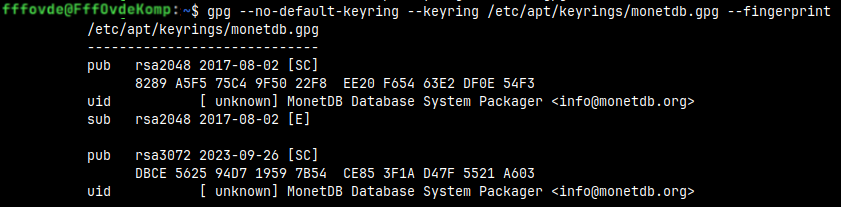
This monetd.gpg file is a binary file. We can read its content with the command: gpg --no-default-keyring --keyring /etc/apt/keyrings/monetdb.gpg --fingerprint
--no-default-keyring #This means that we will not read other GPG keys. --keyring /etc/apt/keyrings/monetdb.gpg #We will read only this GPG key. --fingerprint #Because GPG key is binary file, we will only read its textual presentation, its "fingerprint". #This fingerprint is a long hexadecimal number.
If result of this command is equal to " DBCE 5625 94D7 1959 7B54 CE85 3F1A D47F 5521 A603" for MonetDB, then that means that we have installed the correct key. There is also a key "8289 A5F5 75C4 9F50 22F8 EE20 F654 63E2 DF0E 54F3", but that key is for versions of MonetDB older than 11.49.
Adding a Repository Where MonetDB is Stored
Next, in folder "/etc/apt/sources.list.d" we will create a file with the name "monetdb.list".
#jump to that folder cd /etc/apt/sources.list.d #create new file, you will be asked to provide password sudo touch monetdb.list
Inside of this file we must place this text. These are addresses to MonetdDB repository.
deb [signed-by=/etc/apt/keyrings/monetdb.gpg] https://dev.monetdb.org/downloads/deb/ focal monetdb deb-src [signed-by=/etc/apt/keyrings/monetdb.gpg] https://dev.monetdb.org/downloads/deb/ focal monetdb
We can add this text by running these two lines in our terminal:
Now we can install MonetDB. First, we will update our list of available software with the command:
sudo apt update
Then we can install MonetDB server and client: sudo apt install monetdb5-sql monetdb-client
Creating a DBfarm
In MonetDB, databases are located inside a folder usually called "DBfarm". In addition to the databases, in this folder we will find configuration files with settings for the DBfarm.
Monetdbd, linux daemon, is used to initialize DBfarm by placing configuration files inside it. We use this daemon for changing DBfarm settings and for communication with databases. Monetdbd manages DBfarm and its databases.
monetdbd create /home/fffovde/DBfarm1
We will use "monetdbd" to create a DBfarm on our disk.
Inside of this folder, a new file ".merovingian_properties" will appear. ls -A /home/fffovde/DBfarm1
The Merovingian dynasty was the ruling family of the Franks from the mid-5th century until 751. This dynasty ruled the Netherlands, the country from which MonetDB originates. MonetDB is using this term for some of its internal files and commands.
If we look inside of this file, we will find only one property. All other properties are using default values. We can read those default values by command: monetdbd get all /home/fffovde/DBfarm1
property
hostname
dbfarm
status
mserver
logfile
pidfile
loglevel
sockdir
listenaddr
port
exittimeout
forward
discovery
discoveryttl
control
passphrase
snapshotdir
snapshotcompression
mapisock
controlsock
value
FffOvdeKomp
/home/fffovde/DBfarm1
no monetdbd is serving this dbfarm
unknown (monetdbd not running)
/home/fffovde/DBfarml/merovingian.log
/home/fffovde/DBfarml/merovingian.pid
information
/tmp
localhost
/50000
60
proxy
true
600
no
<unset>
<unset>
.tar.lz4
/tmp/.s.monetdb.50000
/tmp/.s.merovingian.50000
Now, that DBfarm is created, I will start the daemon. We can use daemon to control DBfarm.
monetdbd start /home/fffovde/DBfarm1
Inside of the DBfarm1, we now have 4 files: ls -A /home/fffovde/DBfarm1
File ".merovingian_lock" is empty. This file probably just signalizes that this is DBfarm.
File "merovingian.pid" has the number 1863. This is the number of monetdbd process. If we use command "sudo ss -tlnp" to show us all listening ports, we will see the name monetdbd beside process 1863, and this process will listen the default port 50000.
We can also read content of the log file.
cat /home/fffovde/DBfarm1/merovingian.log
Creation of a Database
While monetdbd is used to manage DBfarm, "monetdb" console application is used to manage individual databases. In the background, "monetdb" will send our commands to monetdbd, and monetdbd will be the one exercising direct control over databases. So, we control databases from "monetdb", but through the power of monetdbd.
This is how we create a database with the name "voc": monetdb create voc
A folder with the name "voc" will appear inside of the DBfarm1 directory.
When database is created, it will only have one default user. That user is administrator "monetdb", and he has default password "monetdb". Database will be created in the maintenance mode. That means that only administrator will be able to start the database, and only on the local computer.
Administrator should create the database with this command. Then he should log into database, and he should change his default password to some other secret and complex password. We will not do that this time, we will continue using the default password "monetdb".
I will change the mode of the database, and I will take it out of the maintenance mode. We can do this to make database available to all the users ( although we currently don't have other users ). monetdb release voc
We can start our database. After the database start, it will be ready for users to log in. monetdb start voc We can check the status of the database with the command: monetdb status
The process with our database server is called "mserver5". This process will run when the database is opened: pgrep mserver5
This command will return process ID of our database server process.
Logging into Database
Now that our database is working and is listening on port 50000, we can try to use it. We will now use another application, with the name "mclient". Let's first recapitulate three console applications used by MonetDB:
"monetdbd" is managing DBfarm.
"monetdb" is managing individual database, with the help of "monetdbd".
Database will run as a "mserver5" process. We'll use "mclient" application to send queries to this process.
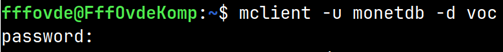
We will login to the "voc" database as a "monetdb" user. Password is the default password "monetdb". mclient -u monetdb -d voc
This will be our welcome screen. We will get "sql>" prompt. There we can type our queries.
I can run this query in my database: SELECT 'columnValues' as columnName;
We can exit the "mclient" program by typing the word "quit".
How to Stop our Server?
This is how we can stop "mserver5" process, the process of the Monetdb database. monetdb stop voc
Log file will tell us what happened. tail -1 /home/fffovde/DBfarm1/merovingian.log
We can put our database in maintenance mode at any time. It doesn't matter if database is opened or closed. We use "lock" command. monetdb lock voc
Next time, only administrator, on the local computer, can start the database with "monetdb start voc" command. He can start the database in exclusive mode, so that he can run some maintenance operations on the database ( he can do backup, or he can make changes in the schema ). We saw previously that database can be taken out of maintenance mode with "monetdb release voc" command. After that, any user can login to a database.
We can also stop "monetdbd" daemon.
monetdbd stop /home/fffovde/DBfarm1
Log file will show us that daemon has stopped.
Install MonetDB in Alternative Way
This time I will jump to the newer version of the Ubuntu. It is "noble". cat /etc/os-release | grep VERSION_CODENAME
Then, I will go the web page https://www.monetdb.org/downloads/deb/repo/. On this web page we have a list of the newest versions of the Ubuntu and Debian. One of the versions is "noble". Enter that folder, click on "monetdb-repo.deb". Firefox will download this file.
We will install this "monetdb-repo.deb" package. sudo apt install /home/fff/Downloads/monetdb-repo.deb
This package will add the file "monetdb.sources" inside of the "/etc/apt/sources.list.d". This file has the same content as the file "monetdb.list" that we have created by hand during the original installation.
This "monetdb-repo.deb" package will also provide GPG keys that can be found on this location "/usr/share/keyrings/monetdb-1.4.gpg". We now understand that we can prepare our computer for monetdb installation by using this package, instead of doing everything by hand.
I will uninstall MonetDB on the "noble" server. We will first create and start a DBfarm, because I want to show you the whole process.
For uninstallation process, if monetdbd is running, we must stop it.
monetdbd stop /home/fff/DBfarm1
We will now list all the packages that have "monetdb" in their name. dpkg -l | grep monetdb
We will remove all those packages. When we delete "monetdb-repo", files with repositories and gpg keys will also be deleted. sudo apt purge libmonetdb-client28 libmonetdb-mutils libmonetdb-stream28 libmonetdb30 monetdb-client monetdb-repo monetdb-server monetdb-sql monetdb5-sql
We will clean all the possible remains: sudo apt autoremove sudo apt autoclean
We still have "monetdb" group and user. cat /etc/passwd | grep monetdb getent group monetdb
We will delete the group and the user. sudo deluser monetdb sudo delgroup monetdb Actually, when we delete the user, the group will also be deleted, so we don't have to delete it separately.
This will not delete DBfarms, only MonetDB application.
Systemd Unit File is a file with settings that Systemd will use when starting and controlling some daemon. From version 11.53.13, MonetDB is using a new systemd file that allows us to change the default directory ( DBfarm ) for databases that are controlled by Systemd.
Old Systemd Unit File
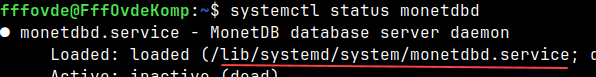
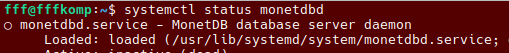
systemctl status monetdbd This command will show us where is systemd unit file for Monetdbd daemon. /lib/systemd/system/monetdbd.service
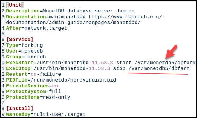
cat /lib/systemd/system/monetdbd.service
The old system unit file was hard coded to always use the directory "/var/monetdbd5/dbfarm". Only databases located within this directory could be controlled by systemd. Only such databases could be started automatically after the computer boots.
[Unit] Description=MonetDB database server daemon Documentation=man:monetdbd https://www.monetdb.org/documentation/admin-guide/manpages/monetdbd/ After=network.target
From version 11.53.13, we have a new system file that allows us to change DBfarm folder, controlled by Systemd.
systemctl status monetdbd This command will show us where is systemd unit file for Monetdbd daemon. /usr/lib/systemd/system/monetdbd.service
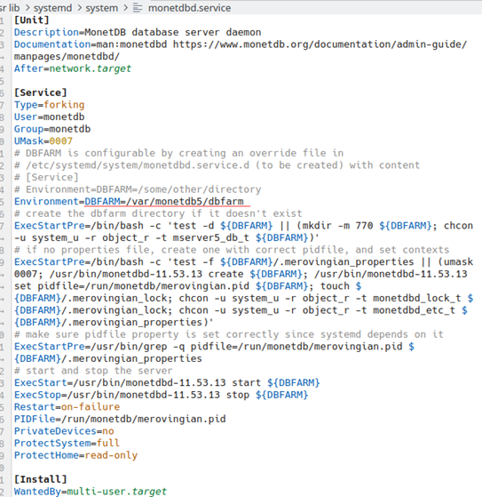
cat /usr/lib/systemd/system/monetdbd.service
This is the new look of the Systemd unit file. We can notice that now we have environ variable DBFARM that is directed to directory "DBFARM=/var/monetdb5/dbfarm" by default. This file is now more complex because it allows us to take some other directory for the DBfarm.
[Unit] Description=MonetDB database server daemon Documentation=man:monetdbd https://www.monetdb.org/documentation/admin-guide/manpages/monetdbd/ After=network.target
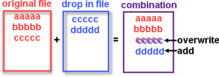
We will not change the original Systemd unit file. Instead of that we will create a "drop-in". That means that we will create another file that will be "amendment" to the original file. "Drop-in" file augments or overrides parts of a unit file without touching the original unit file.
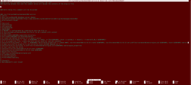
We create this "drop-in" file by running the command: sudo systemctl edit monetdbd
An instance of Nano text editor will open. Inside of it we will se the whole original Systemd unit file, but all the lines will be commented out (every line will start with #).
This location will override the original "/var/monetdb5/dbfarm" location.
I am using linux distribution "KDE Neon". This distribution doesn't use "SELinux". "SELinux" is security feature of the "Red Hat" distribution. The original Systemd unit file provided by the MonetDB developer team is using the command "chcon" that is only useful for the distributions that are using SELinux. I will exclude this code from my Systemd unit file.
Extraordinary, because I am using distro without SELinux, I will also add these corrected lines to my "drop-in" Systemd unit file.
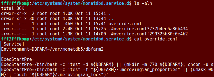
# First, we will delete all of the "ExecStartPre=". ExecStartPre= # This line will add the first part of the "ExecStartPre=". The line "ExecStartPre" is split into three parts, # just to make it more readable. These three lines can be considered as one script. ExecStartPre=/bin/bash -c 'test -d ${DBFARM} || (mkdir -m 770 ${DBFARM})' # This line will add the second part of the "ExecStartPre=". ExecStartPre=/bin/bash -c 'test -f ${DBFARM}/.merovingian_properties || (umask 0007; /usr/bin/monetdbd-11.53.13 create ${DBFARM}; /usr/bin/monetdbd-11.53.13 set pidfile=/run/monetdb/merovingian.pid ${DBFARM}; touch ${DBFARM}/.merovingian_lock)' # Third line is unchanged. ExecStartPre=/usr/bin/grep -q pidfile=/run/monetdb/merovingian.pid ${DBFARM}/.merovingian_properties
This config snippet will be "amendment" to original Systemd unit file. This snippet must be added above the comment "Edits below this comment will be discarded".
We will save this change with "Ctrl+O" ENTER, and then we will exit with the "Ctrl+X". After that we must reload all the systemd unit files.
sudo systemctl daemon-reload
The Changes We Made
This command will show us the new value of the DBFARM environ: systemctl show monetdbd | grep ^Environment=
On the image we use these commands to check override.conf:
cd /etc/systemd/system/monetdbd.service.d ls -alh cat override.conf
systemctl cat monetdbd
This command is also useful because it will show us the original file, and it overrides, and their locations, all together.
Testing The Changes
Because we are going to use Systemd, we should add our user to "monetdb" group.
sudo usermod -aG monetdb "$USER"
After that, we should log out and then log in.
newgrp monetdb
Sometimes log out/in will not be enough. In that case, try to open a new session ( a tab ) in a terminal, or run this command in the existing session. This is happening because OS will try to recycle the old session, so changes are not applied.
We will now create one database and after that we will restart our computer to see if it will be started automatically.
-- Start monetdbd daemon controlled by systemd. -- Create a database. -- Make database available. --Make monetdbd to start automatically after computer reboot. -- Restart our computer.
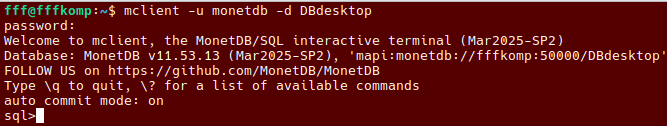
After the reboot, I will open the terminal, and I will try to log in: mclient -u monetdb -d DBdesktop
It will work. We don't have to start the daemon manually.
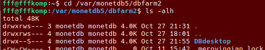
The last step is to check if DBdesktop is really inside of the dbfarm2 directory. cd /var/monetdb5/dbfarm2 ls -alh
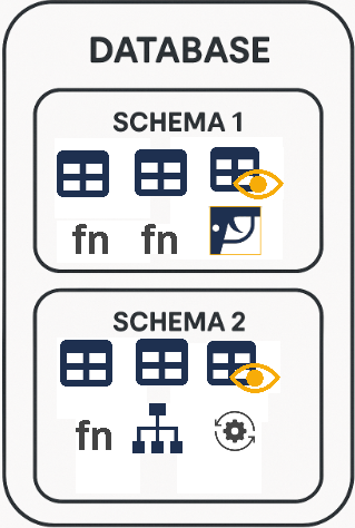
What is Schema
Database is made of tables, views, indices and so on. Inside of Database, each of these objects belongs to some schema. Database is organizationally divided into schemas. There is no overlap between schemas. Some special objects are outside of a schema, like roles.
Usage and modification of schema elements is strictly done by the user or the role that owns that schema. During creation of a schema, we should decide who will be the owner, because later it will not be possible to change ownership. If we want several people to maintain one schema then we should set a role as an owner of a schema.
Only 'monetdb' user and 'sysadmin' role are allowed to create new schemas.
Schema as a File
We can create a file that will contain all the instructions the server needs to create database objects inside of the schema. This file would tell the database which tables, relations, indexes, views to create. In this way, we can create everything that makes up one schema. That is why we call such a file a "schema file". Although we have not learned all the SQL commands needed to create such a file, we can use the "schema file" that the MonetDB development team has prepared for us.
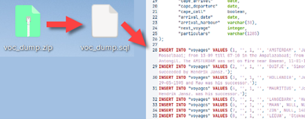
First, we will download sample database from this location:
This will give us ZIP file. Inside of it, there is SQL script with the schema for our new database.
Creation of a New User
For our schema we will create a new user. First, we will enter mclient with 'monetdb' privileges. > monetdbd start /home/fffovde/DBfarm1 > mclient -u monetdb -d voc--password monetdb
For creation of a user, we need username (USER), password (WITH PASSWORD), user's full name (NAME), and default schema for that user (SCHEMA). The default schema is schema that MonetDB will use as a current schema when the user log in. For tables in the current schema, the user can type "SELECT * FROM Table1", but for tables in NON current schemas, the user must type "SELECT * FROM schema.Table1".
"sys" schema is a built-in schema in MonetDB. We will use it temporarily so we can create a new user. sql> CREATE USER "voc" WITH PASSWORD 'voc' NAME 'VOC Explorer' SCHEMA "sys";
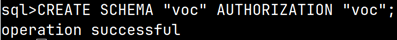
As a 'monetdb' administrator we can create a new schema. We will say that previously created "voc" user is the owner of that schema.
sql> CREATE SCHEMA "voc" AUTHORIZATION "voc";
Don't get confused. The name of our database is "voc", but the name of the new schema is also "voc", and the name of the user is "voc".
We will set the new schema as the default schema for our user. sql> ALTER USER "voc" SET SCHEMA "voc"; sql> \q-- we can exit mclient with "quit" or "\q"
Since the "voc" schema is the default schema for the "voc" user, this schema will be active when this user logs in to MonetDB. Everything the user does will be reflected in this schema, unless the user explicitly mentions that they want to work in a different schema.
Populating our Schema with Database Objects
Our "voc" schema is currently empty, but we have definitions of all the tables, view, indices … inside of our downloaded SQL script. We will use that script to populate our schema. We type:
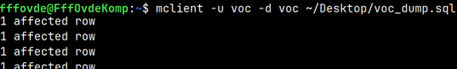
> mclient -u voc -d voc ~/Desktop/voc_dump.sql
This code will log "voc" user into "voc" server. It will also execute all the SQL commands from the "voc_dump.sql" file. When the user log in, and his default schema is "voc", that means that he will log in into "voc" schema. All the SQL commands will be executed inside of this schema.
We will log in again: mclient -u voc -d voc#password is voc
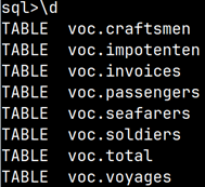
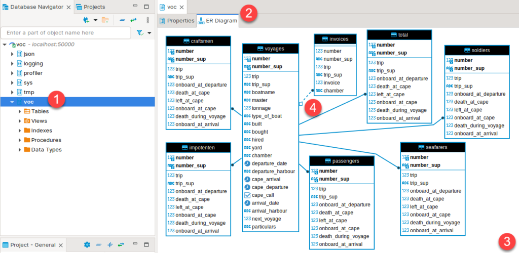
We can use mclient command "\d" to list all the tables and views inside of our database. sql> \d TABLE voc.craftsmen TABLE voc.impotenten TABLE voc.invoices TABLE voc.passengers TABLE voc.seafarers TABLE voc.soldiers TABLE voc.total TABLE voc.voyages
This is what we would get:
DBeaver Database Manager Program
We will install DBeaver database manager program to peruse our database. > sudo snap install dbeaver-ce
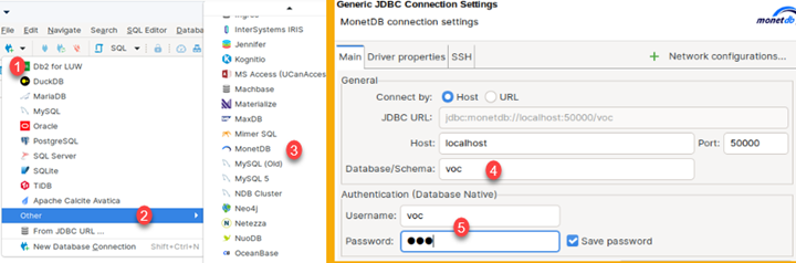
This program is GUI program, so we will open it in our desktop environment. In the program we will click on the triangle (1), and then we will select "Other" (2) to open other servers. There we will find MonetDB. We will click on it (3), and a new dialog will open. In this dialog, host and port are already entered. We just need to enter Database/Schema (4), Username and Password (5) (which is "voc").
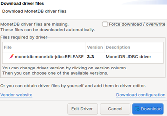
DBeaver will not have driver for MonetDB database installed, so it will offer you to download it. Just accept that offer.
At the end, objects of our database will appear inside of pane on the left side of a program. There, we should double click on schema name (1). After that we can select tab "ER Diagram" (2). There, after some rearrangement, we will see ER diagram of our database (3). As we can see, tables are organized in star schema with "voyages" table as the only fact table. All tables are connected with foreign key constraints, where foreign key is also primary key inside of dimension tables. The only exception is Invoice table where foreign key columns are not primary key columns, and that is why that relationship is shown with dashed line (4).
Here is download for voc_dump.zip file used in this blog post:
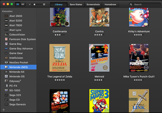
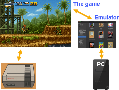
People used to love playing games on old game consoles. People would continue to play those games, but those consoles are no longer for sale, so there are no devices available on which to play these old games.
To solve this problem, emulators are born. Emulators are programs that you install on your computer, and they imitate retro game consoles. In that way, people can still play their favorite video games, even without the game console.
Emulator is simulating the actual hardware. For video games it doesn't matter if they are running on an emulator or on the real device.
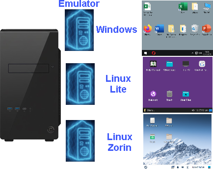
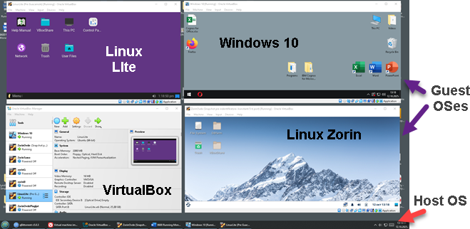
It is also possible to emulate Operational System with all the programs on that system. It is just like we have several computers inside of the one computer case.
Emulator for OS is called hypervisor. One such hypervisor is VirtualBox. VirtualBox is application that we install on our computer, and then we create "virtual machines". A virtual machine (VM) is a software-based emulation of a physical computer that runs its own operating system and applications. With VirtualBox, we can use virtual machines like any other application.
Container
Container is something in between portable application and virtual machine.
Portable application
Container
Virtual machine
– Application that doesn't need installation. – It should match OS version. – Lightest and fastest. – Not isolated from other applications.
– Application with most of its dependencies. – It should match class of OS (Linux, Windows…). – Middle weight. – Mostly isolated.
– Full OS with all the applications. – Should match hypervisor. – Heavy weight. – Fully isolated.
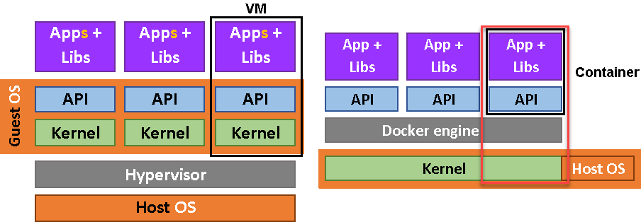
We could say that container is stripped down virtual machine. If we limit virtual machines to only one application, and we force virtual machines to share kernel with the host machine, then we would get containers.
VM – kernel – other apps = container
Containers doesn't use hypervisor. They use docker engine. Docker engine is just an application, just like VirtualBox.
Containers are similar to portable applications, they can be easily deployed, moved, and upgraded. In addition, containers are isolated from other applications and will not compete for resources between them. Containers are much lighter and faster than virtual machines. Containers are immutable, so it is not possible to update parts of the container. This gives us consistency that we can rely on.
Usage of a Container
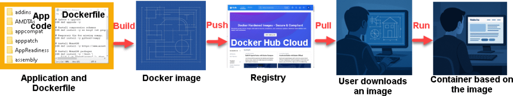
Images are templates used to create containers. An image contains everything needed to build a single container. Images are created by application developers. A developer would create an image and then provide it to users, who would then be able to create containers based on the image.
Let's say we want to publish our application as an image. We will package all our source code along with a "Dockerfile" (explained later) into a single folder. We would use the "Build" command to create a "Docker image". The image is the template from which containers are built. We will upload that image to a Docker image repository (registry). "Docker hub" is a well-known cloud image registry. Users can download our image from the registry. Based on that image, the user will launch the container. In the container, the user would find the application we created.
Anatomy of a Dockerfile
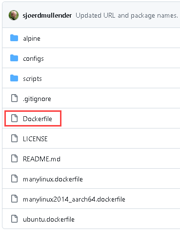
If we go to this git hub web page "link", we will find an example of files that are needed to create an image for MonetDB.
Here we can see source files for MonetDB, and among them there is a file with a name "Dockerfile". This file is an instruction for docker image creation.
"Dockerfile" for MonetDB is a more complex one, so I will show you another one that is simple. =>
"Node.js" is a framework for making web applications. The Dockerfile below is instructions on how to make docker image based on the "Node.js" application.
"FROM" command will download stripped down linux distro from the "Docker Hub" cloud. That stripped linux distro will give system API for our application. After that, we will define working folder, we will copy our application into that folder, and we will install all dependencies for our app. The last line will start our application when a user starts the container.
FROM node:22-alpine# ALPINE is a tiny linux distro, with node.js installed. WORKDIR /app # we set the working directory inside of the ALPINE linux. COPY . .# we copy from the current directory on the host # machine to "/app" directory inside of the ALPINE linux. RUN npm install # we install dependencies that are listed inside of our project, into image CMD npm start# this command will run when our container starts.
All Dockerfiles are made like this. They usually have the same steps:
1) get linux image for API
2) define a folder
3) copy your application
4) download dependencies
5) build/compile
6) create user
7) expose network ports
8) set some environs
9) define startup command
Docker file is basically a list of steps we would take on a physical machine to make our application operational. We will not go any deeper into docker technology. In this article we will only learn how to install docker and download and use MonetDB container.
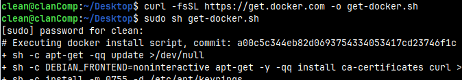
On the bottom of that page, we will find a script. We can download and run this script. That means that we can install docker with two lines of code: curl -fsSL https://get.docker.com -o get-docker.sh sudo sh get-docker.sh
We should add our user to docker group. sudo usermod -aG docker $USER
After that we should log out and log in.
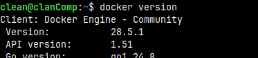
We can now confirm that docker is installed: docker version
Monetdb Container Installation
Getting a Monetdb Image
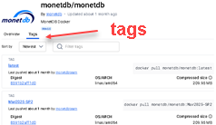
MonetDB containers are hosted on "Docker Hub". MonetDB team will create a new container for each new version of MonetDB. We can find a list of all the MonetDB versions on this page: https://hub.docker.com/r/monetdb/monetdb/tags
The name of each version is made of three elements: nameOfDockerHubAccount/nameOfApplication :versionNumber
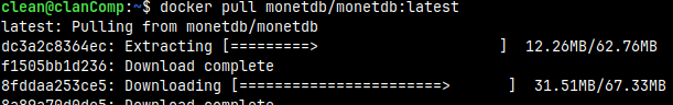
We can download the latest version to our computer using this command. docker pull monetdb/monetdb:latest
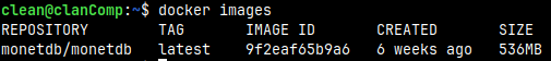
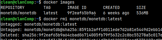
We type this command to observe our images. In non-compressed state, our image is 536 MB. docker images
"Tag" is a version of the image. If we don't provide a tag, we will always get the "latest" version.
Starting MonetDB Container
This is how we can start MonetDB containers. ALPINE linux will expose the server on the default port 50.000, but we must tie that to the host port number. We will use again 50.000 for the host port number. By default, our farm will be on location "/var/monetdb5/dbfarm" inside of the container. The name of default database will be "monetdb". We can set an environ with administrator password like "-e MDB_DB_ADMIN_PASS=monetdb2".
docker run -p50000:50000--restart unless-stopped -e MDB_DB_ADMIN_PASS=monetdb2 monetdb/monetdb:latest
The server will stay in the foreground in the terminal. We will open a new tab inside terminal and there we will type: docker ps #this will list opened containers
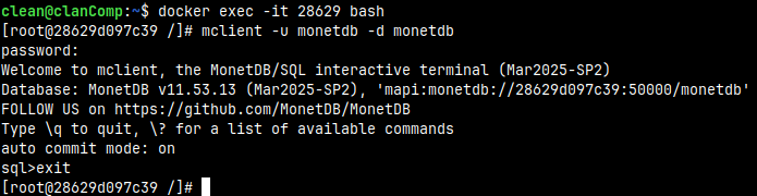
We can connect to bash in the new container. "28629" are start figures of the container ID. We will be connected as a root. docker exec -it 28629 bash
Administrator is "monetdb", and the default database is "monetdb". Password is "monetdb2" and it is set through environ MDB_DB_ADMIN_PASS.
mclient -u monetdb -d monetdb # monetdb2 is password
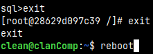
What Will Happen If We Reboot Computer
I will exit bash, and then I will reboot my computer. We used option below with the "docker run" command. This option will make our container to automatically start when the computer starts. It is only possible to stop it manually. --restart unless-stopped If we don't want container to start automatically, we use the default "--restart no".
After restart "docker ps" command will show containers active on our computer. We can see that our container STATUS is "Up 43 seconds".
If we type "docker ps -a" we would get all the containers on our computer, both stopped and active.
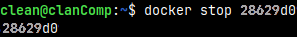
I will stop the container. docker stop 28629
There are now no active containers, just one stopped container.
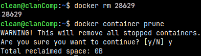
We can now delete stopped container: docker rm 28629
This command would delete all the stopped containers: docker container prune
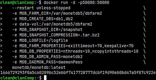
We will now start the container again, but with fully customized options.
Above we use the "-d" option to detach our container. This means that after we run this command, docker will not remain in the foreground, but we will get the command line again, so we can continue typing commands in the same shell.
At the bottom of the image, we can see ID of the new container.
1666729293f….
MDB_FARM_DIR and MDB_CREATE_DBS
We can define in which directory in the container our farm will be created. That is defined with MDB_FARMDIR. With MDB_CREATE_DBS, we can create one or several databases. Between the names of databases there must be no spaces, just the comma.
I will again enter container's bash to check whether we have this folder and databases.
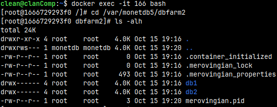
docker exec -it 166 bash
Inside of the bash I will jump do "dbfarm2" folder. cd /var/monetdb5/dbfarm2
Inside this folder we will find databases db1 and db2. ls -alh
We don't have explicitly define MDB_FARM_DIR and MDB_CREATE_DBS. They can take the default values.
/var/monetdb5/dbfarm
monetdb
Volume
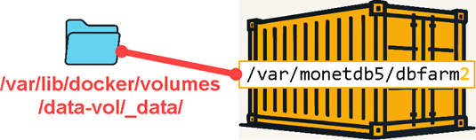
We used option that will create volume. Volume is folder on the host system that is mounted into file system of the container.
-v data-vol:/var/monetdb5/dbfarm2
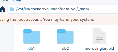
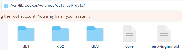
Volumes can be found on the host system at the location: /var/lib/docker/volumes
We can open this folder on our host computer, and inside of it we will find our databases. The purpose of the volumes is to provide data persistence. If our container is deleted, everything inside of it will be deleted. But this will not happen if the data is on the host computer and is only mounted to container.
If we want the data to be safe and persistent, we should use volumes.
MDB_SNAPSHOT_DIR, MDB_SNAPSHOT_COMPRESSION and MDB_LOGFILE
We set MDB_LOGFILE to be "/logfile". That is where is MonetDB log: cat /logfile
By default, logfile will be placed inside of the DBfarm, and will have a name "merovingian.log".
We have set snapshot options: -e MDB_SNAPSHOT_DIR=/snapshot -e MDB_SNAPSHOT_COMPRESSION=.tar.bz2
I will make a snapshot with the default settings:
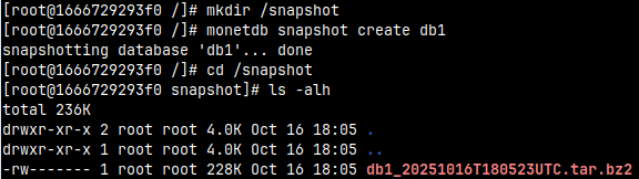
monetdb snapshot create db1
MonetDB will try but will fail because "/snapshot" directory doesn't exist. We must create it.
mkdir /snapshot
monetdb snapshot create db1
cd /snapshot
ls -alh
Snapshot will be created with the assigned compression "bz2".
Snapshots cannot be created if we don't provide snapshots environs. It would be wise to place snapshots inside of the volume to preserve them.
MDB_FARM_PROPERTIES and MDB_DB_PROPERTIES
With MDB_FARM_PROPERTIES environs we set two DBfarm properties. monetdbd get all /var/monetdb5/dbfarm2 | egrep 'exittimeout|keepalive'
Possible properties are explained inside of this blog post "link". We cannot set properties "listenaddr, control and passphrase". "Listenaddr" is always set to "all". "Passphrase" is set by the environ MDB_DAEMON_PASS. If we set MDB_DAEMON_PASS, then "control" will be set to true.
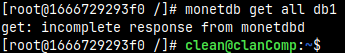
If I try to read database properties with "monetdb get all db1", I am getting an error "incomplete response from monetdb". I don't know why this is happening. We are also kicked out from the bash. This is a bug.
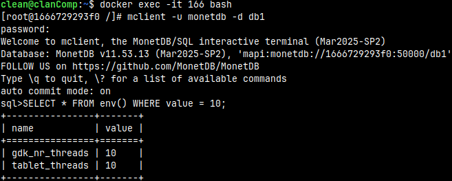
Alternatively, we can read from the system function "env()". I will login again into bash and then into mclient.
docker exec -it 166 bash
mclient -u monetdb -d db1  #password monetdb2
SELECT * FROM env() WHERE value = 10;
In the "env()" table, we can see that the values of the "nthreads" and "ncopyinthreads" properties are set.
Possible properties for a database are explained in this blog post "link".
MDB_DB_ADMIN_PASS and MDB_DAEMON_PASS
MDB_DB_ADMIN_PASS is a mandatory environ. We must set it in order to run MonetDB container.
MDB_DAEMON_PASS is a password for remote Monetdbd control. Remote control of a daemon is explained in the blog post "link". In the context of the containers, this password will allow us to control the daemon in the container from the host operating system.
I will run this command from the host OS to control monetdbd daemon inside of the container. monetdb -h localhost -P daemonPass create db3
For this to work we need to have some conditions fulfilled on the host operational system: – We must have MonetDB installed on the host computer. – DBfarm must be started. Without that we cannot use "monetdb" command. – DBfarm on the host computer must use port number different than the port number of the MonetDB inside of the container.
monetdbd get port /home/clean/DBfarm1
Host computer has Monetdbd on the port 50.0001.
On the host computer we can visit "volume" folder. Inside of it we will see that the new database "db3" has been created.
How to Stop and Start Container?
We can stop the container with command: docker stop 16667 docker ps -a
We can start the container with the command: docker start 16667 docker ps
Clean Up
Deleting Images and Containers
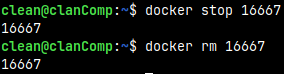
I will now delete everything we have done. First, I will stop and delete container. docker stop 16667 docker rm 16667
We can also delete the image: docker images docker rmi 9f2e
Removing Docker from Your System
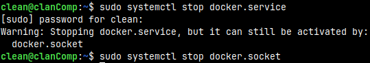
Deleting Docker includes these steps:
We will first stop docker services. sudo systemctl stop docker.service sudo systemctl stop docker.socket
We can now uninstall all parts of the docker: sudo apt purge -y docker-ce docker-ce-cli containerd.io docker-buildx-plugin docker-compose-plugin
In the next step, we will remove docker repository and GPG key. sudo rm -f /etc/apt/sources.list.d/docker.list sudo rm -f /etc/apt/keyrings/docker.gpg
We can update the list of available packages. sudo apt update
We will remove orphaned dependencies. sudo apt autoremove -y sudo apt autoclean
We can also remove all the remaining docker files. sudo rm -rf /var/lib/docker sudo rm -rf /var/lib/containerd sudo rm -rf /etc/docker sudo rm -rf ~/.docker
We will delete docker user group. sudo groupdel docker
Now, we can conclude that docker is deleted: docker --version