Unpivot by using pivot table
This technique is only useful for unpivoting tables with smaller number of columns. Power Query is preferable for larger tables.
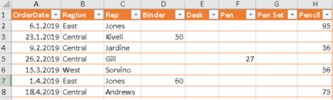
We have a table with a pivoted column of office products. We want to unpivot that column.
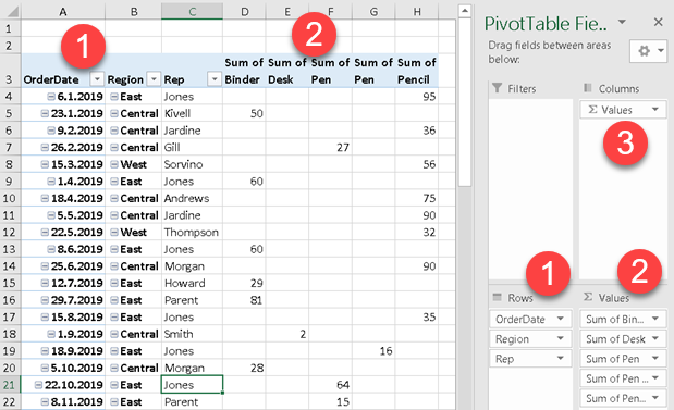
All we have to do is to create a normal Pivot table. In this pivot table all unchanged columns should be placed into Rows section (1). All other columns, that should be unpivoted, should be placed in Values section (2). Notice that in Columns section we have a special column "∑ Values" (3), that Excel created itself.
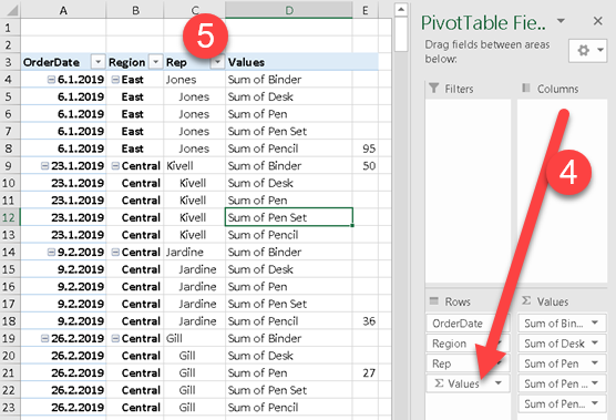
Now drag that special "∑ Values" column into Rows section (4). We will immediately get unpivoted table (5). This table asks for some maintenance so is best to make a copy of it in spreadsheet and then fix its header, and filter rows with no values.
This approach could will not be optimal when there are many columns that should be unpivoted. In that case we have to move all those columns into Values section manually. This could be tedious. In that case it is much easier to use Power Query unpivot tool.
Unpivot by using Power Query
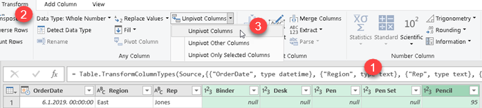
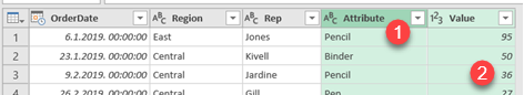
Get your unpivoted table into Power Query. Select all columns that should be unpivoted (1). In Transform tab (2) find command "Unpivot Columns" (3). This command will do all the work. Notice that we also have command "Unpivot Other Columns" (3). This allow us to select only columns that shouldn't be unpivoted, and then all the other columns will be unpivoted. When we have really big number of columns to unpivot, this command make it even more easier to accomplish our task.
At the end we get unpivoted table. Again, we have to fix column names (1). Rows without vales will be automatically filtered (2).
Excel sample file:
Instructional video: