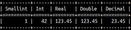
We know that there are 9 number data types ( tinyint, smallint, int, bigint, hugeint, decimal, double, float, real ). If we want to convert some value to these data types, we can use CAST and CONVERT functions.
SELECT CAST(true as smallint) AS "Smallint",
       CONVERT(42, int) AS "Int",
       CONVERT(123.45, real) AS "Real",
       CAST('123.45' as double) AS "Double",
       CAST(23.45 as decimal(5,2)) AS "Decimal";
Arithmetic Operators
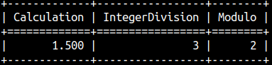
We can always make our calculation by using operators + , – , * , / or modulo %.
SELECT 0 + 1 * 4 - ( 5.0 / 2 ) AS "Calculation",  -- 5.0 / 2 = 2.5 because of decimal
       7 / 2 AS "IntegerDivision",   -- 7 / 2 = 3 because of INT
       8 % 3 AS "Modulo";
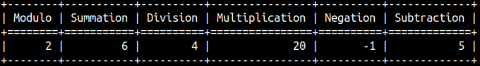
Arithmetic operators have their counterpart in arithmetic functions:
SELECT mod( 8, 3 ) AS "Modulo",
       sql_add( 3, 3 ) AS "Summation",
       sql_div( 8, 2 ) AS "Division",
       sql_mul( 4, 5 ) AS "Multiplication",
       sql_neg( 1 ) AS "Negation",
       sql_sub( 7, 2 ) AS "Subtraction";
Bitwise Operators and Functions
We already know operators AND, NOT, OR and XOR. We used them with TRUE and FALSE values. In MonetDB, instead of TRUE and FALSE we can use 1 and 0.
SELECT TRUE AND FALSE;
SELECT 1 AND 0;-- we'll get the same result
If we have two binary numbers, then we can apply AND, NOT, OR and XOR on each of their zeros and ones. That is how bitwise operators work.
Number1
1
0
1
0
1
Number2
1
1
1
0
0
————
————
————
————
————
————
Num1 AND Num2
1
0
1
0
0
Num1 OR Num2
1
1
1
0
1
Num1 XOR Num2
0
1
0
0
1
NOT Num1
0
1
0
1
0
Instead of typing binary numbers, we will show them as regular integers. This is how we use bitwise operators and functions:
Bitwise operator
Bitwise function
Result
AND
SELECT 91 & 15;
SELECT BIT_AND( 91, 15 );
11 -- 01011011 AND 00001111 = 00001011
OR
SELECT 32 | 3;
SELECT BIT_OR( 32, 3 );
35 -- 00100000 OR 00000011 = 00100011
XOR
SELECT 17 ^ 5;
SELECT BIT_XOR( 17, 5 );
20 -- 00010001 XOR 00000101 = 00010100
NOT
SELECT ~1;
SELECT BIT_NOT( 1 )
-2 -- NOT 00000001 = 11111110
Bitwise Shift
Bitwise left shift is when we add a zero on the right side of a binary number. Each time we add another zero, the value of a number is increased double.
00000001  <<   1   =   00000010
SELECT 1 << 1;  -- 2
00000001  <<   2   =   00000100
SELECT 1 << 2;   -- 4
00000001  <<   3   =   00001000
SELECT 1 << 3;    -- 8
It is similar, if we remove one figure from the the right side. Then we have a right shift. Each right shift will reduce number to its half.
00001000 >> 1 = 00000100 SELECT 8 >> 1; -- 4
00000100 >> 1 = 00000010 SELECT 4 >> 1; -- 2
00000010 >> 1 = 00000001 SELECT 2 >> 1; -- 1
Beside using operators, we also have functions that can do bitwise shift.
SELECT left_shift(1, 2);
SELECT right_shift(8, 1);
Min and Max
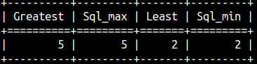
To calculate the larger/smaller value of two values, we can use the functions "largest" and "smallest". The functions "skl_max" and "skl_min" are just synonyms of the previous two functions.
SELECT greatest( 4, 5 ) AS "Greatest",
       sql_max( 4, 5 ) AS "Sql_max",
       least( 2, 100 ) AS "Least",
       sql_min( 2, 100 ) AS "Sql_min";
Taking a Root
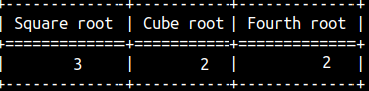
For root calculation we have two functions. One is for square root, and the other one is for the cube root.
SELECT SQRT( 9 ) AS "Square root", CBRT( 8 ) AS "Cube root", POWER( 16.0, 1.0 / 4 ) AS "Fourth root";
If we need to calculate a root of a higher order, then we can use mathematical property . In the last column we calculated the fourth root of a 16 by using this property. For this transformation we had to use POWER function.
Logarithm and Exponential Functions
SELECT POWER( 2, 5 ); --32
This function will raise a number to the power of another number.
SELECT exp(3); -- 20,08553692
We can define this function based on POWER function, because exp(3) = POWER(e,3), where e is Euler number (approximately 2.71).
The opposite function of POWER function is a logarithm. If POWER( b, x ) = Y, then log( b, Y ) = x:
SELECT POWER( 2, 3 ) AS "Power", LOG( 2, 8 ) AS "Logarithm";
If we are working with an Euler number, then we can use LOG function without its first argument (or we can use its alias LN function):
SELECT LOG( 20.08553692 ) AS "Log", LN( 20.08553692 ) AS "Ln" ;
We also can use functions LOG10( x ) or LOG2( x ), which are just shortcuts for LOG10( x ) = LOG( 10, x ) and LOG2( x ) = LOG( 2, x ).
Ceiling and Floor Functions
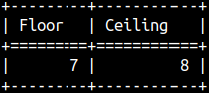
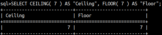
For each real number N, we can say that it is between two nearest integers. Those two integers we call ceiling and floor. We have SQL functions with such names, they will return us those two nearest integers:
SELECT FLOOR( 7.55 ) AS "Floor", CEILING( 7.55 ) AS "Ceiling";
For CEILING function, we can use its alias CEIL.
Each integer is floor and ceiling for itself.
Rounding and Truncating
We can reduce the number of decimal places in two ways. We can just cut off the excess decimals using the truncate function. The second argument will decide how many decimal places to trim.
SELECT sys.ms_trunc( -5.628, 0 ) AS "No decimals", sys.ms_trunc( –5.628, 1 ) AS "One decimal", sys.ms_trunc( -5.628, 2 ) AS "Two decimals";
Another approach is to round the number. The second argument will again decide how many decimal places will survive. If the last decimal is 5, we will always round up (in absolute value).
SELECT ROUND( 5.5, 0 ) AS "No decimals", ROUND( -5.55, 1 ) AS "One decimal", ROUND( 5.555, 2 ) AS "Two decimals";
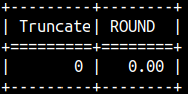
If the second argument is negative, the result will be zero.
SELECT sys.ms_trunc( 9.99, -2 ) AS "Truncate", ROUND( 9.99, -3 ) AS "ROUND";
There is also a function that does truncation first and then rounding. SELECT sys.ms_round( 5.546, 2, 1 ), --5.546 => 5.54 (truncate) => 5.54 (rounded) sys.ms_round( 5.546, 2, 0 ); --5.546 => 5.546 (no truncate) => 5.55 (rounded)
Creating Random Numbers
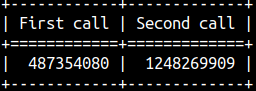
Each time we call RAND() function, we will get random integer between 0 and 2,147,483,647 ( 231-1 ). SELECT RAND() AS "First call", RAND() AS "Second call";
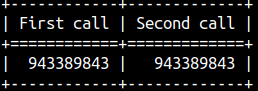
RAND() function can accept seed argument. The seed argument will allow us to get the same random value every time. SELECT RAND(77) AS "First call", RAND(77) AS "Second call";
Other Mathematical Functions
SELECT ABS( -5 ); --to calculate an absolute value
SELECT SIGN( -5 ), SIGN( 5 ); -- to find out the sign of a number
SELECT sys.alpha(5.0, 1.2);
This function is for astronomy. compute alpha 'expansion' of theta for a given declination (used by SkyServer)
Trigonometric and Hyperbolic Functions
SELECT PI(); will return 3.14.
This is one right triangle. The smallest of its angles is 36.87°.
To transform this angle to radians we can use RADIANS function. For transforming it back we will use DEGREES function.
SELECT RADIANS( 36.87 ); --returns 0.6435, that is 36.87 * ( 3.14 / 180 )
SELECT DEGREES( 0.6435 ); --returns36.87, that is 0.6435 * ( 180 / 3.14 )
SELECT SIN( 0.6435 );
Sine function will return the ratio b/c = 3/5 = 0.6. It accepts an angle value in radians, as do all the functions below.
SELECT COS( 0.6435 );
Cosine function will return the ratio a/c = 4/5 = 0.8.
SELECT TAN( 0.6435 );
Tangent function will return the ratio b/a = 3/4 = 0.75.
SELECT COT( 0.6435 );
Cotangent function will return the ratio a/b = 4/3 = 1.33.
Then we have inverse functions:
SELECT ASIN( 0.6 ); -- 0.6435
If we know that b/c = 0.6, then arcsine function will tell us that the angle is 0.6435 radians.
SELECT ACOS( 0.8 ); -- 0.6435
If we know that a/c = 0.8, then arccosine function will tell us that the angle is 0.6435 radians.
SELECT ATAN( 0.75 ); -- 0.6435
If we know that b/a = 0.75, then arctangent function will tell us that the angle is 0.6435 radians.
SELECT ATAN( 3, 4 ); -- 0.6435
The same ATAN function will also work with dividend and divisor ( 3/4 = 0.75 ).
Offset functions are window functions that return a value from a specified row. The row is determined as an offset from the reference point. There are two major reference points. The first is the current row, the second is the frame border. Based on this, we distinguish between "row offset functions" and "frame offset functions".
Row Offset Functions
With row offset functions, we move from the current row several steps up or down. Our movement is dependent only on the current row, so we do not use frames with row offset functions. Frames are not applicable in this case.
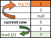
LAG function will move us up. LEAD function will move us down.
We will create one sample table so that we can observe how these functions work.
CREATE TABLE offsetTable( "Month" INT, Value INT );
LAG function will allow us to get some previous value and to place it in the current row. That would allow us to compare some old and some new value, so we can analyze the change in time. SELECT "Month", Value, LAG( Value, 2 ) OVER ( ORDER BY "Month" ) FROM offsetTable ORDER BY "Month";
We can see three drawbacks in the image above:
Month April doesn't have a value. LAG function doesn't notice that, and will happily move two rows above, but not two months before. For the fifth month we are getting the value from the February which is three months before, not two. That is the consequence of the missing month April. We should avoid using LAG function when we are missing some time points.
For months January and February, we have nulls in the new column . Previous values don't exist so we have to be satisfied with nulls.
In the third row, the Value column has NULL. Sometimes we want to go over those nulls and not count them as steps we take. There is a way to achieve this in SQL standard, but that part of SQL standard is not implemented in MonetDB, so null values will always be counted as one step. Subclause IGNORE NULLS is not supported.
--not supported SELECT "Month", Value, LAG( Value, 2) IGNORE NULLS OVER (ORDER BY "Month" ) FROM offsetTable ORDER BY "Month";
LAG can work with partitions.
We should always order rows inside partition with ORDER BY. Although LAG function can work without ORDER BY, the results will be unpredictable and meaningless.
LAG Function Arguments
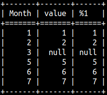
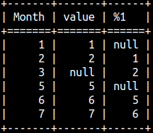
If the second argument is missing, then the default value is 1. In the image, we can see that the rows are shifted by one row.
SELECT "Month", Value, LAG(Value) OVER (ORDER BY "Month") FROM offsetTable ORDER BY "Month";
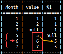
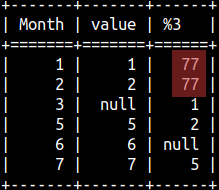
Only if we provide second argument, we can also provide the third argument. The third argument is the default value. Default value will be used for those rows where previous values don't exist. SELECT "Month", Value, LAG(Value,2,77) OVER (ORDER BY "Month") FROM offsetTable ORDER BY "Month";
Default value has to be of the proper data type that match other values in the column.
Third argument is optional. If we skip it, the default value would be null.
SELECT "Month", Value, LAG(Value,2) OVER (ORDER BY "Month") FROM offsetTable ORDER BY "Month";
LEAD Function
LEAD function is the same as LAG function, just the opposite. Notice that we can achieve the same result with LEAD function, as with LAG function, if we change ORDER BY from ascending order to descending order.
SELECT "Month", Value, LAG(Value,1) OVER (ORDER BY "Month" ASC) FROM offsetTable ORDER BY "Month";
SELECT "Month", Value, LEAD(Value,1) OVER (ORDER BY "Month" DESC) FROM offsetTable ORDER BY "Month";
<=== totally the same ===>
This is similar example. Both statements use ASC, but the result is the same. This is because the offset argument can be negative. This is another way we can make the LAG and LEAD functions do the same thing.
SELECT "Month", Value, LAG(Value,2) OVER (ORDER BY "Month" ASC) FROM offsetTable ORDER BY "Month";
SELECT "Month", Value, LEAD(Value,-2) OVER (ORDER BY "Month" ASC) FROM offsetTable ORDER BY "Month";
<=== totally the same ===>
Frame Offset Functions
For frame offset functions everything is relative to frame borders. We have three functions of this type. – FIRST_VALUE will return the first value in the frame. – NTH_VALUE will return the NTH value in the frame, from the start of a frame. – LAST_VALUE will return the last value in the frame.
For frame offset functions, we always need to have frame. If 6 is the month in the current row, then the frame is between 4th and 8th month. Now that we know the frame size and position, it is easy to see that the first value in this frame is 5.
SELECT "Month", Value, FIRST_VALUE(Value) OVER (ORDER BY "Month" RANGE BETWEEN 2 PRECEDING AND 2 FOLLOWING) FROM offsetTable ORDER BY "Month";
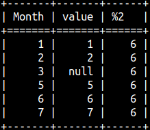
If we omit frame definition, the default frame RANGE BETWEEN UNBOUNDED PRECEDING AND CURRENT ROW will be used. Be aware of this and always define frame.
SELECT "Month", Value, LAST_VALUE(Value) OVER (ORDER BY "Month") FROM offsetTable ORDER BY "Month";
Frame offset functions can work with partitions.
We should always order rows inside frame with ORDER BY. Frame offset functions can work without ORDER BY, but the results will be unpredictable and meaningless.
NTH_VALUE Function
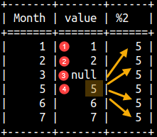
NTH_VALUE function has another argument which tells how many steps to move from the start of a frame. In the example bellow, our frame is the whole partition. Fourth number in the "value" column is number 5. That number will be the result of this window function. SELECT "Month", Value, NTH_VALUE(Value,4) OVER (ORDER BY "Month" ASC RANGE BETWEEN UNBOUNDED PRECEDING AND UNBOUNDED FOLLOWING) FROM offsetTable ORDER BY "Month";
If the second argument is omitted, default value will not be one, but the error will be raised.
The value of that second argument can not be negative.
We can use partitions with NTH_VALUE. You should always provide frame definition, and you should have ORDER BY for your frame.
Difference From SQL Standard
IGNORE NULLS is not supported in MonetDB for the functions FIRST_VALUE, LAST_VALUE and NTH_VALUE.
With IGNORE NULLS we would be able to not count nulls, but this is not supported in MonetDB. SELECT "Month", Value, NTH_VALUE(Value,3) IGNORE NULLS --not supported OVER (ORDER BY "Month" ASC RANGE BETWEEN UNBOUNDED PRECEDING AND UNBOUNDED FOLLOWING) FROM offsetTable ORDER BY "Month";
NTH_VALUE can not use subclause FROM LAST. This would allow to count steps from the end of the frame, and not from the start. But this is not supported in MonetDB.
SELECT "Month", Value, NTH_VALUE(Value,2) FROM LAST --not supported OVER (ORDER BY "Month" ASC RANGE BETWEEN UNBOUNDED PRECEDING AND UNBOUNDED FOLLOWING) FROM offsetTable ORDER BY "Month";
We actually don't need "FROM LAST" subclause. It is enough to change ORDER BY to descending, and we would get the same result as with "FROM LAST". SELECT "Month", Value, NTH_VALUE(Value,2) OVER (ORDER BY "Month" DESC RANGE BETWEEN UNBOUNDED PRECEDING AND UNBOUNDED FOLLOWING) FROM offsetTable ORDER BY "Month";
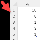
For each row in Excel we know its row number. On the image we can see that in Excel, in front of column "A", we have a "column" with row numbers.
We can create the same column, with row numbers, in MonetDB, by using ROW_NUMBER() window function. There are two more similar functions in MonetDB, and those are RANK() and DENSE_RANK().
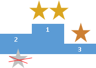
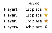
Sometimes, in Olympic games, two sport players can share gold medal. In that case, there is no silver medal. Next best player will get bronze medal. This is called "olympic ranking". In MonetDB we can create such ranking with RANK() function.
For apples we wouldn't apply Olympic ranking. Instead of that we would place apples of the similar quality in consecutive classes, so we would have apples of first, second and third class. This can be achieved with DENSE_RANK() function. As it's name implies, DENSE_RANK() doesn't have gaps in ranking, so there will be always someone who will get silver medal.
With ROW_NUMBER(), RANK() and DENSE_RANK(), we can not use frames. These functions are not returning one value for each row, and because of that frames are not applicable. These functions always work with the whole partitions.
This is an example for all of the three functions:
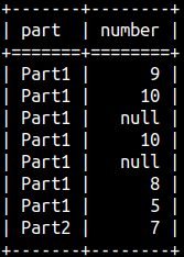
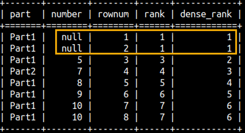
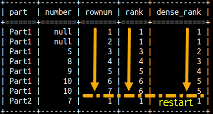
SELECT part, number,
   ROW_NUMBER() OVER(ORDER BY Number) AS rowNum,
   RANK() OVER (ORDER BY Number) AS Rank,
   DENSE_RANK() OVER(ORDER BY Number) AS dense_Rank
FROM rankFunctions
ORDER BY Number;
From this example we can conlude: 1) All null values are treated as the same value. 2) It is important to use "ORDER BY" inside of WINDOW function, without it result would be meaningless. 3) These three functions are not taking any arguments.
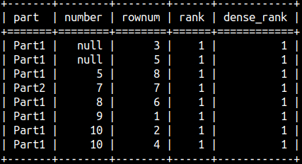
This is what would be the result without ORDER BY. RANK and DENSE_RANK functions would return one's, so they are not really working without ORDER BY.
ROW_NUMBER() function can be still be useful without ORDER BY. It can be used as a column that would deduplicate rows that are otherwise indistinguishable.
SELECT part, number,
   ROW_NUMBER() OVER() AS rowNum,
   RANK() OVER () AS Rank,
DENSE_RANK() OVER() AS dense_Rank FROM rankFunctions ORDER BY Number;
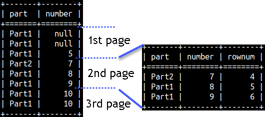
ROW_NUMBER() function is great when we want to read data step by step, by reading N consecutive rows each time. Example on the right would help us read our data by fetching 3 rows each time.
WITH Tab1 AS ( SELECT Part, Number, ROW_NUMBER() OVER (ORDER BY Number) AS RowNum FROM rankFunctions ) SELECT * FROM Tab1 WHERE RowNum BETWEEN 4 AND 6;
Process of reading N by N rows is called pagination. We are reading one page at a time.
Partitioning would just mean that we are restarting the sequence.
SELECT part, number, ROW_NUMBER() OVER(PARTITION BY Part ORDER BY Number) AS rowNum, RANK() OVER (PARTITION BY Part ORDER BY Number) AS Rank, DENSE_RANK() OVER(PARTITION BY Part ORDER BY Number) AS dense_Rank FROM rankFunctions ORDER BY Part, Number;
Relative Ranking Functions
Relative ranking functions will show us rank of a row expressed in normalized way, with numbers between 0 and 1. There are two relative ranking functions. Those are CUME_DIST() and PERCENT_RANK().
CUME_DIST() function
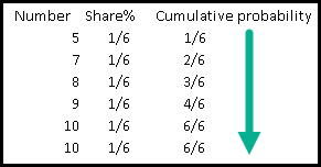
CUME_DIST() is short for Cumulative Distribution. This function will can answer questions like: What percentage of screws (image on the right) is equal or smaller than 9 cm?
The answer would be 4/6, that is 66%.
This function is called cumulative because it shows a cumulative probability.
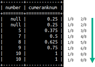
This would be the result for our sample table. SELECT Number, CUME_DIST() OVER(ORDER BY Number) AS cumeRankNum FROM rankFunctions ORDER BY Number;
PERCENT_RANK() function
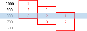
For PERCENT_RANK() function, we will start with an example. We can see that RANK() of Number will return numbers 1,1,3,4,5,6,7,7. PERCENT_RANK() function is similar, just the values are normalized, so it will return numbers from 0 to 1.
SELECT Number, RANK() OVER (ORDER BY Number) AS rankNum, PERCENT_RANK() OVER(ORDER BY Number) AS percRankNum FROM rankFunctions ORDER BY Number;
PERCENT_RANK() will calculate it's values with this formula:
PERCENT_RANK() will exclude current row from the calculation, like it doesn't exist.
NTILE(n) Function
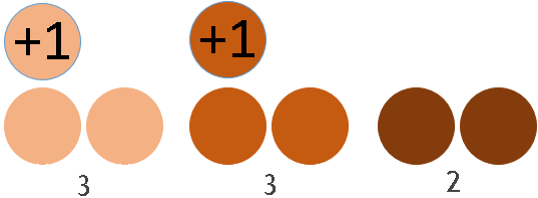
We have 6 screws.
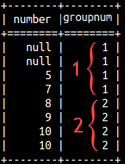
We want to divide them into 2 groups. This is the most natural way to divide them:
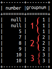
This is if we want to divide them into 3 groups:
Such separation of elements into groups can be done in SQL with NTILE(n) function. We will use NTILE(2) to divide Number column into 2 groups and NTILE(3) to divide Number columns into 3 groups.
SELECT Number, NTILE(2) OVER(ORDER BY Number) AS groupNum FROM rankFunctions ORDER BY Number;
SELECT Number, NTILE(3) OVER(ORDER BY Number) AS groupNum FROM rankFunctions ORDER BY Number;
We can notice that nulls would be considered as the smallest values. We can also notice that on the first image we have 2 groups with 4 Numbers. That is perfect. But, on the second image we have three groups with 3,3,2 Numbers. Groups are not of equal size. In that case we would start with 2,2,2 groups, of equal size, but the first few groups would get an extra Number. That would make things almost perfect.
Final Conclusion
General rules for ranking functions are this:
1) All null values are treated as the same value. 2) It is important to use "ORDER BY" inside of WINDOW function, without it result would be meaningless. 3) None of the ranking functions is taking an argument, with the exception of NTILE(n) function. 4) None of these functions can work with frames, but they can use partitioning. 5) If values for several rows are the same, then the values returned by ranking functions will be the same for those rows. In our sample table, both of two rows with Number 10 will always have the same rank, no matter what ranking function we are using (except ROW_NUMBER() ).
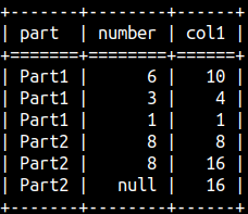
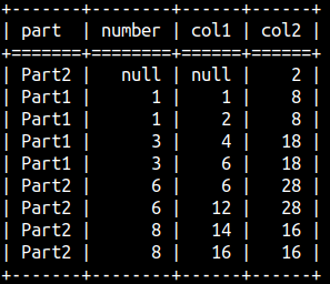
Aggregate functions support partitioning, ordering and framing. Below we can see example of this.
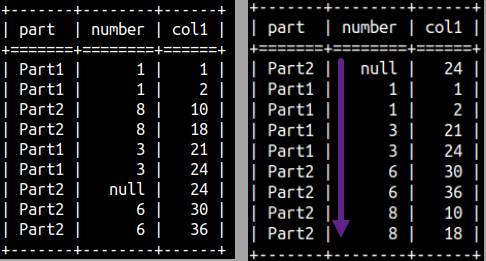
SELECT Part, Number, SUM( Number) OVER ( PARTITION BY Part ORDER BY Part DESC, Number NULLS LAST ROWS BETWEEN UNBOUNDED PRECEDING AND CURRENT ROW ) As Col1 FROM aggWindow ORDER BY Part, Number DESC;
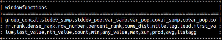
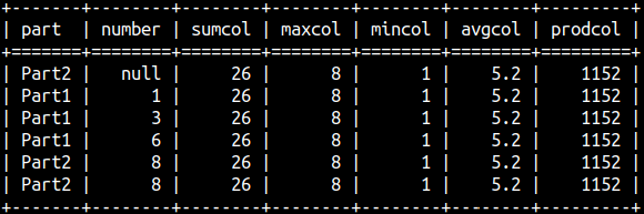
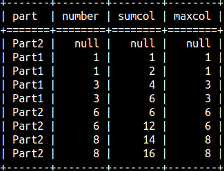
We can use WINDOW definition to show all of the classical aggregation functions. Our window is defined as (), so we will aggregate the whole column.
SELECT Part, Number,
       SUM( Number ) OVER W AS SumCol,
MAX( Number ) OVER W AS MaxCol, MIN( Number ) OVER W AS MinCol, AVG( Number ) OVER W AS AvgCol, PROD( Number ) OVER W AS ProdCol FROM aggWindow WINDOW W AS ( ) ORDER BY Number;
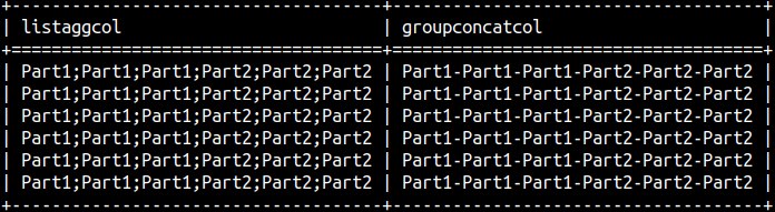
We can use listagg and group_concat functions to concatenate text from our column.
SELECT listagg( Part, ';' ) OVER W AS listAggCol, group_concat( Part, '-' ) OVER W AS groupConcatCol FROM aggWindow WINDOW W AS ( );
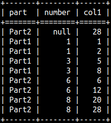
Running Aggregations
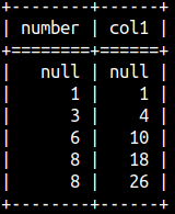
Aggregate functions are used to calculate cumulative values. In this case we create our frame relative to current row and we use ORDER BY.
SELECT Number, SUM( Number ) OVER ( ORDER BY Number ROWS BETWEEN UNBOUNDED PRECEDING AND CURRENT ROW ) As Col1 FROM aggWindow;
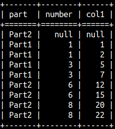
Moving Aggregations
We can also use aggregate functions for calculation of moving aggregations.
SELECT Number, AVG( Number ) OVER ( ORDER BY Number ROWS BETWEEN 1 PRECEDING AND CURRENT ROW ) As Col1 FROM aggWindow;
Usage of window functions in ORDER BY
Window functions can be used only after all data from our query is created. That means that Window functions can be used only in SELECT and ORDER BY clauses. Here is the usage of Window function in ORDER BY.
SELECT Part, Number FROM aggWindow ORDER BY COUNT(Number) OVER (PARTITION BY Part);
Combining WINDOW functions and GROUPBY clause
If we combine WINDOW functions and GROUP BY clause, there is a difference between what these functions can see. GROUP BY calculation can only see one group, but it can see all the detail rows inside of that group. WINDOW function can see all the groups, but it can not see detail rows.
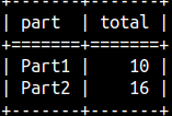
SELECT Part, SUM( Number ) AS Total FROM aggWindow GROUP BY Part ORDER BY Part;
GROUP BY will sum detail rows for each group separately. It can not combine values from different groups.
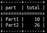
SELECT Part, SUM(SUM( Number )) OVER ( ROWS BETWEEN UNBOUNDED PRECEDING AND CURRENT ROW ) AS Total FROM aggWindow GROUP BY Part ORDER BY Part;
WINDOW function will see only those rows that are returned after GROUP BY finished its calculation. WINDOW function can see only totals for the groups, and not the detail rows. WINDOW function can work with those totals, from all of the groups, at the same time.
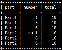
It seems that GROUP BY and WINDOW functions are of equal power. But that is not the truth. WINDOW functions are more powerful. We can preserve detail rows in the original columns, and we can create new columns with aggregated values. This allow us to compare detail and aggregated values. This is not possible with GROUP BY.
Look, we now have detail values and aggregated values in the same row. We can now easily calculate share of details in the total.
SELECT Part, Number, SUM( Number ) OVER ( PARTITION BY Part ) AS Total FROM aggWindow ORDER BY Part, Number;
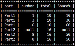
SELECT Part, Number, SUM( Number ) OVER ( PARTITION BY Part ) AS Total, 100 * Number / SUM( Number ) OVER ( PARTITION BY Part ) AS "Share%" FROM aggWindow ORDER BY Part, Number;
The last column will show us share as a percentage.
Statistical Aggregate Functions
Statistical aggregate functions can be used in the same way as the classical aggregate functions.
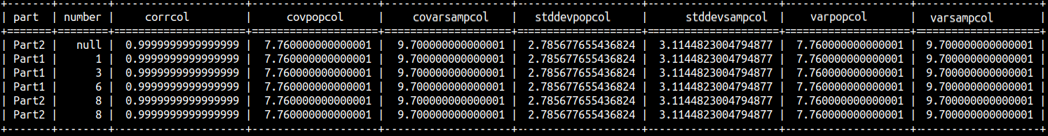
SELECT Part, Number, CORR( Number, Number - 1 ) OVER W AS CorrCol, COVAR_POP( Number, Number - 1 ) OVER W AS CovarPopCol, COVAR_SAMP( Number, Number - 1 ) OVER W AS CovarSampCol, STDDEV_POP( Number ) OVER W AS StdDevPopCol, STDDEV_SAMP( Number ) OVER W AS StdDevSampCol, VAR_POP( Number ) OVER W AS VarPopCol, VAR_SAMP( Number ) OVER W AS VarSampCol FROM aggWindow WINDOW W AS ( ) ORDER BY Number;
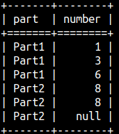
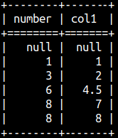
If the parentheses after OVER keyword are empty, then we will aggregate the whole Number column. Aggregate functions, like SUM, AVERAGE, MAX…, will ignore NULLs.
1+1+3+3+6+6+8+8 = 36
SELECT Part, Number,
SUM( Number ) OVER ( ) AS Col1
FROM aggWindow;
Usage of Partitions
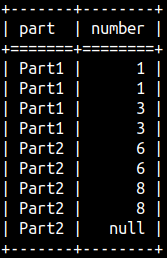
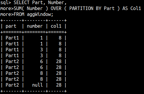
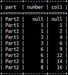
We can partition our table before aggregation. Each partition will be separately aggregated.
1+1+3+3 = 8 6+6+8+8 = 28
SELECT Part, Number,
SUM( Number ) OVER ( PARTITION BY Part ) AS Col1
FROM aggWindow;
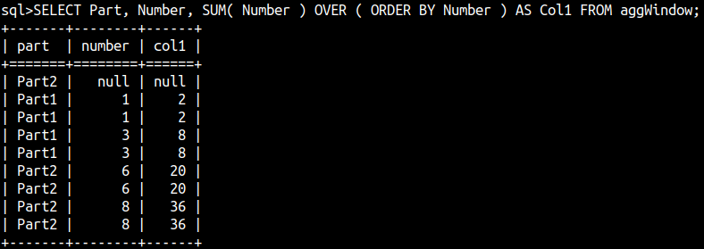
ORDER BY and Frames
ORDER BY is always accompanied with the frame definition. If the frame definition is not provided, then the default frame is used. The default frame is:
RANGE BETWEEN UNBOUNDED PRECEDING AND CURRENT ROW
SELECT Part, Number,
SUM( Number ) OVER ( ORDER BY Number ) AS Col1
FROM aggWindow;
We should avoid using default values and we should always provide explicit frame definitions.
If we don't provide ORDER BY, there is no knowing how frames will be created. It is important to provide ORDER BY to avoid randomness. Notice in the image that we have a meaningless running total, because there is no ordering of the Number column.
SELECT Part, Number, SUM( Number ) OVER ( ROWS BETWEEN UNBOUNDED PRECEDING AND CURRENT ROW ) AS Col1 FROM aggWindow;
If we sort Number column in the final data set, meaningless running total will become more obvious.
SELECT Part, Number, SUM( Number ) OVER ( ROWS BETWEEN UNBOUNDED PRECEDING AND CURRENT ROW ) AS Col1 FROM aggWindow ORDER BY Number;
Notice that ORDER BY clause can exist on two places in the statement. One is used to define frame, and the classic one is used to sort final data set.
SELECT Part, Number, SUM( Number ) OVER ( ORDER BY Number ROWS BETWEEN UNBOUNDED PRECEDING AND CURRENT ROW ) AS Col1 FROM aggWindow ORDER BY Number;
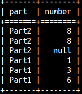
Within the Window, the NULL position can be controlled independently of the ORDER BY clause. We can use NULLS LAST or NULLS FIRST to explicitly define position of NULLs.
SELECT Part, Number, SUM( Number ) OVER ( PARTITION BY Part ORDER BY NumberNULLS LAST ROWS BETWEEN UNBOUNDED PRECEDING AND CURRENT ROW ) AS Col1 FROM aggWindow ORDER BY Number;
In the image, our Null is appearing in the first row because of the classic ORDER BY clause, but it is paired with the biggest value in the "Col1" for Partition 2 (28). NULL is now part of the last frame in the last Partition.
This is because of the clause NULLS LAST,whichchanged position of the NULL row, from the first, to the last, in the window definition.
Examples for the Rows, Ranges and Groups
In this example, frame is defined by the current and two previous rows.
SELECT Part, Number,
SUM( Number ) OVER
( ORDER BY Number
  ROWS BETWEEN 2 PRECEDING AND CURRENT ROW ) AS Col1
FROM aggWindow ORDER BY Number;
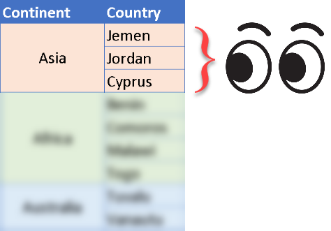
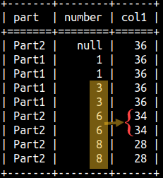
With Ranges, current row comprise all the rows with the same value. Current row is a set of records, and not only one row.
SELECT Part, Number, SUM( Number ) OVER ( ORDER BY Number RANGE BETWEEN CURRENT ROW AND 3 FOLLOWING ) AS Col1 FROM aggWindow ORDER BY Number;
This example will use all the rows with the current value X and will calculate range with limits [X,X+3].
For X = 6, limits are [6,6+3]. Numbers 6 and 8 are both inside of this range.
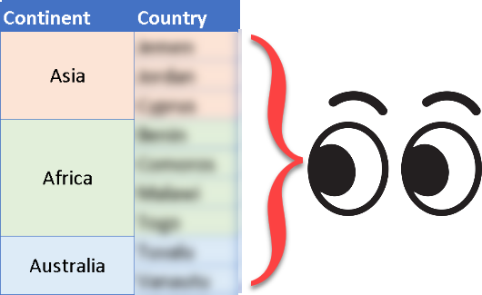
Each frame encompass current group, one previous group, and all the latter groups.
SELECT Part, Number,
SUM( Number ) OVER
( ORDER BY Number
  GROUPS BETWEEN 1 PRECEDING AND UNBOUNDED FOLLOWING ) AS Col1
FROM aggWindow ORDER BY Number;
Window Chaining ( WINDOW clause )
Window functions are verbose. If we want to use them several times in our statement, then our statement will become really long.
SELECT Part, Number, SUM( Number ) OVER ( PARTITION BY Part ORDER BY Number ROWS BETWEEN 1 PRECEDING AND CURRENT ROW ) AS Col1, SUM( Number ) OVER ( ORDER BY Number DESC GROUPS BETWEEN 1 PRECEDING AND CURRENT ROW ) AS Col2 FROM aggWindow ORDER BY Number;
The only workaround is available if we are using the same window for several functions. We can then define our window once, with WINDOW clause, and then reference it several times.
SELECT Part, Number, SUM( Number ) OVER W AS SumCol, MAX( Number ) OVER WAS MaxCol FROM aggWindow WINDOW W AS ( PARTITION BY Part ORDER BY Number ROWS BETWEEN 1 PRECEDING AND CURRENT ROW ) ORDER BY Number;
Default frames
We already saw that we should avoid using default frames. There are two more abbreviations that will assume default frames.
Abbreviated syntax
Full definition of the default frame
{ UNBOUNDED | X } PRECEDING
BETWEEN { UNBOUNDED | X } PRECEDING AND CURRENT ROW
{ UNBOUNDED | X } FOLLOWING
BETWEEN CURRENT ROW AND { UNBOUNDED | X } FOLLOWING
SELECT Part, Number, SUM( Number ) OVER ( ORDER BY Number ROWS1 PRECEDING) AS Col1 FROM aggWindow ORDER BY Number;
--The same is for RANGE or GROUPS.
Default frame is: SELECT Part, Number, SUM( Number ) OVER ( ORDER BY Number ROWSBETWEEN 1 PRECEDING AND CURRENT ROW) AS Col1 FROM aggWindow ORDER BY Number;
--The same is for RANGE or GROUPS.
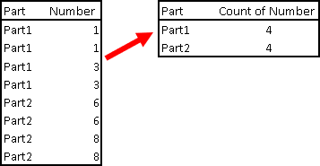
Window Functions and GROUP BY
We can group our table with GROUP BY. After we do this, window function will only see those grouped rows. On the image to the left, window function will only see 2 rows. Detail rows will not be any more available to window function.
The question is, what syntax to use to create running total in this grouped table.
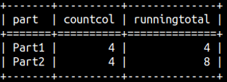
Bellow we can see correct syntax. Columns in the grouped table are referred as Part and COUNT( Number ). Our Window function is based on those columns. That means that our window function will be SUM(COUNT( Number )).
SELECT Part, COUNT( Number ) AS CountCol, SUM(COUNT( Number )) OVER ( ORDER BY Part ROWS BETWEEN UNBOUNDED PRECEDING AND CURRENT ROW) AS RunningTotal FROM aggWindow GROUP BY Part ORDER BY Part;
Limitations of Window Functions
Range and ORDER BY
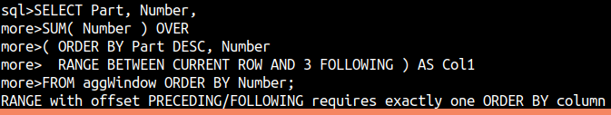
Range frames can only use one column inside of ORDER BY clause.
SELECT Part, Number, SUM( Number ) OVER ( ORDER BY Part DESC, Number RANGE BETWEEN CURRENT ROW AND 3 FOLLOWING ) AS Col1 FROM aggWindow ORDER BY Number;
DISTINCT and Window functions
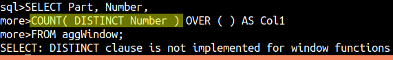
We can not use DISTINCT keyword inside of Window function.
SELECT Part, Number
COUNT( DISTINCT Number ) OVER ( ) AS Col1
FROM aggWindow
;


 This function is for astronomy.
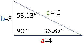
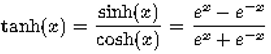 This is hyperbolic tangent.


 <=== totally the same ===>
 <=== totally the same ===>