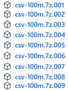
For this benchmark we will use sales data from the fictitious company "Contoso". We can download our database from the github. If we go to this address, we will find there compressed CSV files with the data. In total there are 8 files of 500 MB, and one smaller file with 250 MB ( 4250 MB in total ).
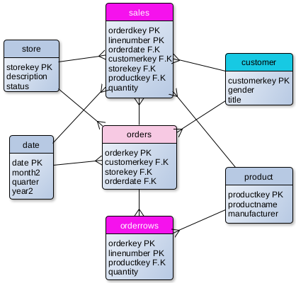
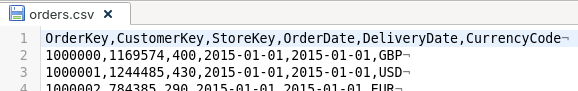
When we unzip these files, inside we will find 8 CSV files. This is sales cube with tables that can show us sales and orders per product, customer, date and store.
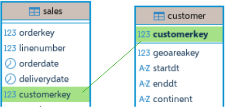
Three big tables are "Orders" ( 88M ), "Sales" ( 211M ) and "OrderRows" ( 211M ). Dimension table "Customer" has 2M rows, and all the other dimension tables are small.
Not all of the columns are shown on the image.
—————————————————————————————— In CSV file "date.csv" I will change the names of columns month=>month2 and year=>year2, because MonetDB will not accept original names. "Month" and "Year" are reserved words.
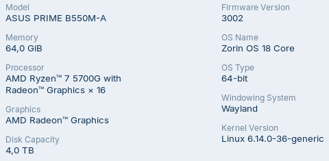
Machine Hardware
For this benchmark we will use CPU with 8 cores and 64 GB of RAM.
Our operational system is Zorin 18.
Creating Tables and Loading CSV Files
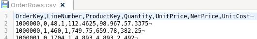
OrderRows Table
CREATE TABLE orderrows (
OrderKey BIGINT NOT NULL,
LineNumber SMALLINT NOT NULL,
ProductKey SMALLINT NOT NULL,
Quantity SMALLINT NOT NULL,
UnitPrice REAL NOT NULL, --DECIMAL(8,4)
NetPrice REAL NOT NULL, --DECIMAL(10,6) UnitCost REAL NOT NULL --DECIMAL(8,4) );
First, I will create table for OrderRows in the MonetDB. I will not create primary and foreign key constraints this time.
I will fill this table from my CSV file with "COPY INTO" statement.
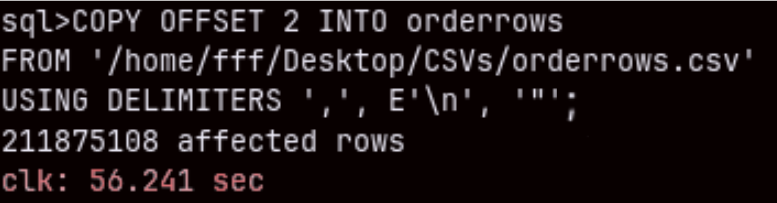
COPY OFFSET 2 INTO orderrows
FROM '/home/fff/Desktop/CSVs/orderrows.csv'
USING DELIMITERS ',', E'\n', '"'
NULL AS '';
Import of this 211M rows table will last only one minute ( 56.241 sec ). Amazing.
Other Tables
I will leave a file for download at the end of this article. That file will have SQL for creation and import of all of the Contoso tables.
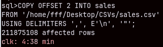
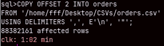
Bellow we can see time for import for two other larger files. Smaller dimension tables are imported almost instantly.
Sales (211M) table will need almost 5 minutes to be imported.
Orders (88M) CSV table will be imported in 62 seconds.
Query Benchmarking
Cold Start
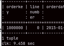
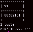
I will now restart my computer. I want to make sure to run a cold query. This simple query bellow will run for 10 seconds. MonetDB database becomes faster as more queries are executed. This ability of MonetDB is called "cracking". MonetDB will automatically sort, group and index columns during the SELECT queries. That will make subsequent queries faster.
SELECT * FROM sales LIMIT 1;
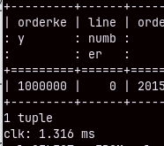
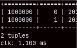
If we run this query again, it will be executed in just 1.3 miliseconds. This is not the result of query caching. If we make a query that takes 2 or 3 rows, we will again see these exceptional speeds.
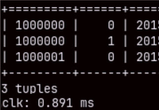
SELECT * FROM sales LIMIT 2; SELECT * FROM sales LIMIT 3;
Aggregated Queries in MonetDB
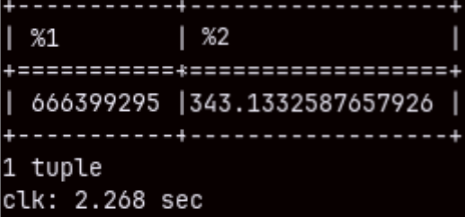
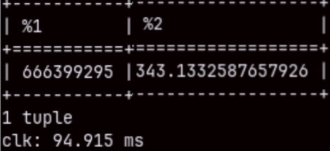
If we aggregate two columns in the "sales" table, that query will touch 211M rows. It will be fast ( 2.268 sec. ), but we can repeat it to get only 94.915 ms.
SELECT SUM( quantity ), AVG( unitprice ) FROM sales;
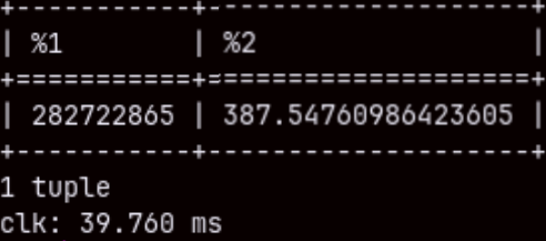
I will run the same query, but this time with a filter. SELECT SUM( quantity ), AVG( unitprice ) FROM sales WHERE orderdate <= '2020-05-25';
We will get the result even faster. This proves that the result is not cached. MonetDB run the query again, but this time "cracking" made our query faster.
It's hard to make a benchmark when execution times are constantly changing. So, from now on I will focus on the fastest times.
How Database Reports Execution Time
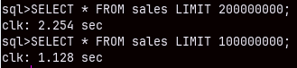
SELECT * FROM sales LIMIT 1000000;--13 ms SELECT * FROM sales LIMIT 2000000; --24 ms
MonetDB is reporting that the second query is slower than the first one. That is something that we are expecting. The problem is that according to my computer clock the first query was finished after 7 seconds, and the second one after 15 seconds.
Databases only report the time spent to produce the results in the memory. It will not include the time needed to print the result in the shell or any other client. That is why MonetDB is reporting 13 ms, but I can see the result only after 7 seconds. MonetDB has command to suppress printing of the result in the shell. I will use that command ( command explained here ) next, to test reading the whole tables.
This is how long it takes MonetDB to read a large number of rows. Columnar databases are better suited for aggregate queries, but we can see that MonetDB is capable of performing OLTP types of queries quite well.
I will disable my command, so we can again see the results of our queries.
Joins
SELECT productkey, SUM( quantity ), AVG( netprice ) FROM sales GROUP BY productkey;
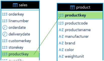
This query will execute for 340 ms. If we want to see brands then we have to make a join between "product" and "sales" tables.
SELECT brand, SUM( quantity ), AVG( netprice ) FROM sales INNER JOIN product ON sales.productkey = product.productkey GROUP BY brand;
The query with a join will last more than 1 second. We can speed it up if we create a foreign key constraint.
Now that we have foreign key constraint, the query from before will become 200 ms faster. That is 20% faster.
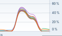
Query from before is a traditional analytical query. If we look at system monitor, we will see that during the execution of this query the load will be equally distributed between CPU cores. MonetDB is capable to significantly parallelize query execution. That means that our individual queries can be speed up with a CPU that has even more cores.
DISTINCT, LIKE, ROLLUP
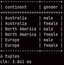
From the table "customer" we can list distinct continents and genders in 3.841 ms.
SELECT DISTINCT continent, gender FROM customer;
We can get distinct combinations of storekey and currency code from "sales" table in half of the second.
SELECT DISTINCT storekey, currencycode FROM sales;
If we want to count unique combinations of the orderkey and currencycode, then our query will be slow, it will last almost 11 seconds. But this query has to count 88 million rows.
SELECT COUNT( * ) FROM
     ( SELECT DISTINCT orderkey, currencycode
       FROM sales );
Query like this will also last 11 seconds.
SELECT COUNT( * ) FROM
  ( SELECT orderkey, currencycode
     FROM sales
     GROUP BY orderkey, currencycode );
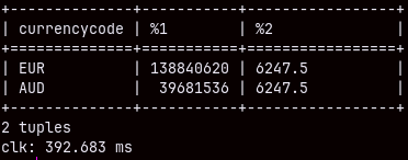
LIKE operator allows usage of the wild cards. Sign "_" will replace one letter.
SELECT currencycode, SUM( quantity ), MAX( unitprice )
FROM sales
WHERE currencycode LIKE '_U_' GROUP BY currencycode;
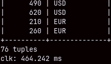
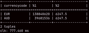
If we use the sign "%" that replaces several characters, then the speed will drop, almost double.
SELECT currencycode, SUM( quantity ), MAX( unitprice )
FROM sales
WHERE currencycode LIKE '%U_' GROUP BY currencycode;
Before we test ROLLUP, I will create foreign key constraint between "customer" and "sales" tables.
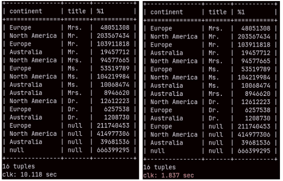
This time we have unusually slow query. It will take full 10 seconds. SELECT continent, title, SUM( quantity ) FROM customer INNER JOIN sales ON customer.customerkey = sales.customerkey GROUP BY ROLLUP( continent, title ); ——————————————————————————————————————————– Query with union would be much better choice for this. Only 1.837 seconds. SELECT continent, title, SUM( quantity ) FROM sales INNER JOIN customer ON sales.customerkey = customer.customerkey GROUP BY continent, title UNION SELECT continent, null, SUM( quantity ) FROM sales INNER JOIN customer ON sales.customerkey = customer.customerkey GROUP BY continent UNION SELECT null, null, SUM( quantity ) FROM sales;
This show us that there is still room for improvements in MonetDB optimizer.
Window Functions
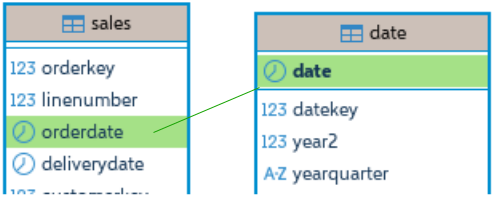
I will first add foreign key constraint between "sales" and "date" tables.
ALTER TABLE date ADD CONSTRAINT date_pk PRIMARY KEY ( date );
ALTER TABLE sales ADD CONSTRAINT FKfromDate FOREIGN KEY ( orderdate ) REFERENCES date ( date );
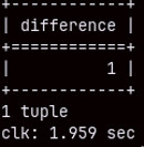
We can use LAG function to compare sales for the current and the previous row. Each value from quantity column will have a pair in the BeforeQty column, except in the first row ( no previous ). Quantity in that first row will make a difference. This query will execute in 2 seconds.
SELECT ( SUM( Qty ) - SUM( BeforeQty ) ) AS Difference FROM
( SELECT Quantity AS Qty,
  LAG( Quantity, -1 ) OVER ( ORDER BY date ) AS BeforeQty
  FROM date INNER JOIN sales ON date.date = sales.orderdate );
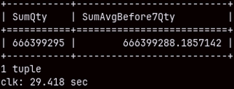
For each row in the table, we will calculate the average quantity of the previous 6 rows and the current row. At the end will see sums of the quantity and these rolling averages. This query will last 29 seconds.
SELECT SUM( Quantity ) AS "SumQty", SUM( AvgBefore7Qty ) AS "SumAvgBefore7Qty" FROM
( SELECT Date, Quantity,
     AVG( Quantity ) OVER
         ( ORDER BY Date ROWS BETWEEN 6 PRECEDING AND CURRENT ROW)
             AS AvgBefore7Qty
FROM date INNER JOIN sales ON date.date = sales.orderdate );
Updates
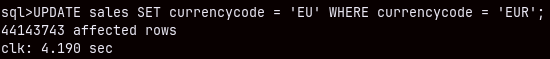
MonetDB should be slow for updates, but it managed to update 44 milion rows for just 4.19 seconds. UPDATE sales SET currencycode = 'EU' WHERE currencycode = 'EUR';
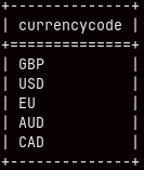
We can confirm that all of the values 'EUR' are updated to 'EU'.
SELECT DISTINCT currencycode FROM sales;
Problematic Queries
Double Grouping
Double grouping is when we first group our data, and then we group that result. For example, we will total sales quantity per customerkey, and then we will count customers per total quantity. We will count how many customers have the same total quantity.
This query is problematic because while the first grouping can be fast, the second one could be much longer. The result of the first grouping will have 2M rows, because we have so much customers. In the second stage, we have to group these 2M rows, and that is when I expect the performance to become bad.
SELECT customer.customerkey, SUM( quantity ) AS TotQty
FROM customer INNER JOIN sales ON customer.customerkey = sales.customerkey
GROUP BY customer.customerkey;
In the first phase I will measure how much time is needed to group by customer. It is 5 seconds because there are 2 million customers.
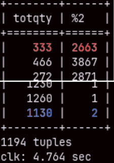
Second phase: SELECT TotQty, COUNT( customerkey ) FROM ( SELECT customer.customerkey, SUM( quantity ) AS TotQty FROM customer INNER JOIN sales ON customer.customerkey = sales.customerkey GROUP BY customer.customerkey ) as FirstPhase GROUP BY TotQty;
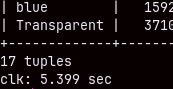
We can see on the image that we have 2,663 customers with total quantity of 333 items, and only two with 1,130 items. The time for execution is again 5 seconds. This is something I didn't expect. I am pleasantly surprised. I can tell you that these kinds of queries are problematic for Power BI database ( SSAS ).
Aggregated Query from Two Fact Tables ( Stitch Query )
This time I will create foreign key constraint on the "OrderRows" (211M) table. I want to aggregate sales and orderrows per product brend. ALTER TABLE orderrows ADD CONSTRAINT FK_Product FOREIGN KEY ( productkey ) REFERENCES product ( productkey );
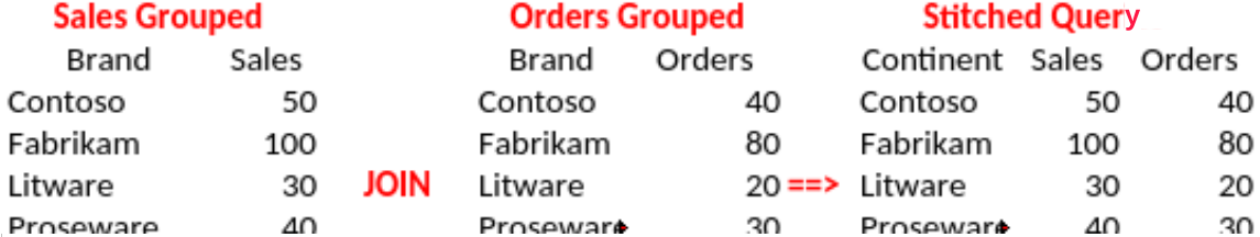
"Stitch" query is when we aggregate two fact tables per the same dimension and we get two data sets as a result. Then we join those two data sets in the final result. This is how we aggregate values from two fact tables.
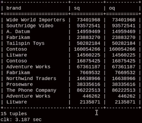
Query bellow will last 7.5 seconds. This is longer than I expected. If we ran subqueries separately the time would be just 900 ms each. Because we only have 15 brands, it is surprising that it will take 5 seconds just to join two small tables. SELECT S.brand, Sq, Oq FROM ( SELECT Brand, SUM( quantity ) Sq FROM Product INNER JOIN Sales ON Product.Productkey = Sales.ProductKey GROUP BY Brand ) S INNER JOIN ( SELECT Brand, SUM( quantity ) Oq FROM Product INNER JOIN Orderrows ON Product.Productkey = OrderRows.ProductKey GROUP BY Brand ) O ON S.Brand = O.Brand;
If we "UNION ALL" our subqueries, the execution will last 7.5 seconds, too. SELECT Brand, SUM( quantity ) Sq FROM Product INNER JOIN Sales ON Product.Productkey = Sales.ProductKey GROUP BY Brand UNION ALL SELECT Brand, SUM( quantity ) Oq FROM Product INNER JOIN Orderrows ON Product.Productkey = OrderRows.ProductKey GROUP BY Brand;
I have tried to read two small subqueries into python, and then to join them with pandas. Python reported execution time of just 1.2 seconds. It is strange that we can get the final result faster by combining MonetDB and Pandas, then just by using MonetDB.
WITH S AS
( SELECT productkey, SUM( quantity ) AS Sq FROM Sales GROUP BY productkey ),
O AS ( SELECT productkey, SUM( quantity ) AS Oq FROM Orderrows GROUP BY productkey ), PS AS ( SELECT brand, SUM( Sq ) AS SQty FROM Product INNER JOIN S ON Product.productkey = S.productkey GROUP BY brand ), PO AS ( SELECT brand, SUM( Oq ) AS OQty FROM Product INNER JOIN O ON Product.productkey = O.productkey GROUP BY brand ) SELECT PS.brand, Sqty, OQty FROM PS INNER JOIN PO ON PS.brand = PO.brand;
We can reduce our fact tables by grouping them by productkey and then following the same logic. This approach would speed up our query to 5.5 seconds.
WITH S AS ( SELECT productkey, SUM(quantity) AS Sq
            FROM sales
            GROUP BY productkey ),
O AS ( SELECT productkey, SUM(quantlty) AS Oq
       FROM orderrows
       GROUP BY productkey )
SELECT P.brand, SUM(S.Sq) AS Sq, SUM(O.Oq) AS Oq
FROM product P
 LEFT JOIN S ON S.productkey = P.productkey
 LEFT JOIN O ON O.productkey = P.productkey
GROUP BY P.brand;
This would be the fastest version of this query. It would execute in only 3 seconds.
In this query, we would use the the last subquery to join reduced sales and orderRows tables, with the product table.
INSERT INTO SELECT
I will use "INSERT INTO SELECT" to make "Sales" table bigger. Before doing that, I will remove FK constraints. I will also change optimizer. ALTER TABLE sales DROP CONSTRAINT fkfromproduct; ALTER TABLE sales DROP CONSTRAINT fkfromcustomer; ALTER TABLE sales DROP CONSTRAINT fkfromdate; SET sys.optimizer = 'minimal_pipe';
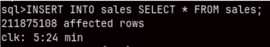
I will now run this statement to make my sales table twice bigger. INSERT INTO sales SELECT * FROM sales; MonetDB needed 5 minutes to do this.
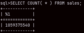
I will do this 1 more time. That will double the number of rows to 844M. That was done in 9:48 minutes. Then, I will again read from the CSV file into this table. That will add another 211M rows, so in total "sales" table will now have one billion rows.
I will recreate foreign key constraint toward "product" table. ALTER TABLE sales ADD CONSTRAINT FKfromProduct FOREIGN KEY ( productkey ) REFERENCES product ( productkey );
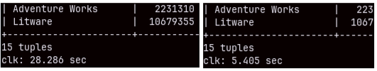
I will run now this query twice. The first time it will end after 28 seconds, and the second time after 5,5 seconds. SELECT brand, SUM( quantity ), AVG( netprice ) FROM sales INNER JOIN product ON sales.productkey = product.productkey GROUP BY brand;
SELECT color, SUM( quantity ), AVG( netprice ) FROM product INNER JOIN sales
    ON sales.productkey = product.productkey
GROUP BY color;
Immediately after, I run the same query, by it was grouped by color. The time was again 5 seconds.
We can see that performance is good, even with 1B rows.
Conclusions
We can conclude some things: – MonetDB is usually very fast. – Initially, until the database worm up, queries can be slow. – We should always set foreign key constraints to achieve speed boost. – Some kinds of queries are better optimized than others.
– MonetDB does not use much memory. During the import of the "sales" table, the RAM usage increased from 4 to 13 GB. It was the same during this last, 1B rows, query. At other times, the usage was much less.