0540 Backing up the MonetDB Database
Database Schema ( as a file )
A database schema is a list of all database objects and their attributes, written in a formal language. If we already have a ubiquitous formal language for creating database objects, SQL, then we should use SQL language for writing our schema.
| If our server understands a particular dialect of SQL, it can read the list of SQL statements and, based on that, can create the entire specified database. Specification is provided as a file with a "*.sql" extension. |  |
| A schema is useful when we want to create a database according to a specification. But we want to back up our database, and for that we need a backup of the data in addition to the schema. We can include INSERT INTO statements with all the data, in a schema. Now we have a file that is an exact symbolic image of our database, and can be used as backup file. |  |
| We already used such file in the blog post about sample MonetDB database "link". This file, with a data, can also be considered as a schema file, in the broader sense. |  |
Qualities of the Good Schemas
| Database objects should be created in the proper order. For example, tables should be created before we create views that are based on those tables. Here we can see recommended order of statements: | a) CREATE SCHEMAS b) CREATE SEQUENCES c) CREATE TABLES d) ALTER TABLES for FOREIGN KEYS e) CREATE INDEXES | f) CREATE VIEWS g) CREATE FUNCTIONS and PROCEDURES h) CREATE TRIGGERS i) INSERT INTO data j) GRANT/REVOKE |
When running schema file, we should wrap it into transaction to avoid incomplete creation.
Credentials
In this blog post "link", I have show you how to create a file with credentials, and we placed it into $HOME folder ( "/home/fffovde" ) on the "voc" server. If we have such file, we don't need to provide credentials, for MonetDB, every time we run some command in the shell.You can notice bellow that I will run my Msqldump commands without providing credentials, by using such file. Users can only backup database objects they have access to, so with administrator account we will be able to backup everything. |  |
Msqldump
Msqldump is a console program used to create a schema from an existing MonetDB database. The resulting file can be used for backups or to migrate the database to another MonetDB server. With some manual tweaking of this file, we can use it to migrate database to a server other than MonetDB (perhaps Postgres or MySQL).
We should redirect the result of this app to the file on our computer.msqldump -d voc > /home/fffovde/Desktop/voc_db.sql |  |
| If we don't, the long schema will go to stdin, and we usually don't want that. |  |
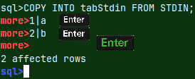
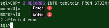
| By default, instead of the INSERT INTO statements, our schema will return "COPY FROM stdin" statements. This will make restoring of the database faster. |  |
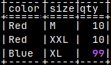
We can use "-e" switch to add NO ESCAPE clause to COPY statement. msqldump -d voc -e > /home/fffovde/Desktop/voc_db.sql |
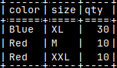
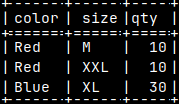
For returning INSERT INTO statements, we should use "-N" switch. msqldump -d voc -N > /home/fffovde/Desktop/voc_db.sql |
Partial Backup of Database
Option "-f" means that we will only backup functions.msqldump -d voc -f > /home/fffovde/Desktop/voc_db.sql |  |
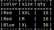
With option "-t", we can backup only one table. We should provide fully qualified name of a table, because default schema for administrator is sys ( we are logged in as administrator ).msqldump -d voc -t voc.invoices > /home/fffovde/Desktop/voc_db.sql |  |
With wild cards we can backup a set of tables with a similar name. This code bellow would return only tables "passengers, seafarers and soldiers".msqldump -d voc -t voc.%ers > /home/fffovde/Desktop/voc_db.sql |  |
With upper letter "-D voc", we will export database without data. msqldump -D voc > /home/fffovde/Desktop/voc_db.sql |  |
Location of A Schema File
We don't have to use redirection to a file. We can use option "-o". msqldump -d voc -o /home/fffovde/Desktop/voc_db.sql |  |
We can export our database to a folder. In that case switch "-O" is using upper letter.msqldump -d voc -O /home/fffovde/Desktop/voc_db_folder |  |
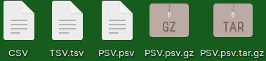
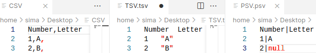
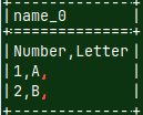
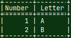
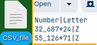
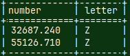
If we export database to a folder, that folder will contain all of the DDL ( data definition language ) statements inside of the "dump.sql" file, but the data will be one separate CSV file for each table. CSV files will not have a header (because we have CREATE TABLE statements in the "dump.sql"), delimiter will be TAB. |  |
Only when we use export to a folder, it is possible to use "-x" option. CSV files will be compressed to that file format. We can use "lz4,gz,bz2,xz".msqldump -d voc -x lz4 -O /home/fffovde/Desktop/voc_db_folder |  |
Credentials in the Command
I will now move my credentials to temporary folder, so from now we will have to provide credentials to Msqldump. mv /home/fffovde/.monetdb /tmp/.monetdb |  |
Name of our user now has to be provided with the switch "-u". msqldump -u monetdb -d voc -o /home/fffovde/Desktop/voc_db.sql |  Password is always provided separately. |
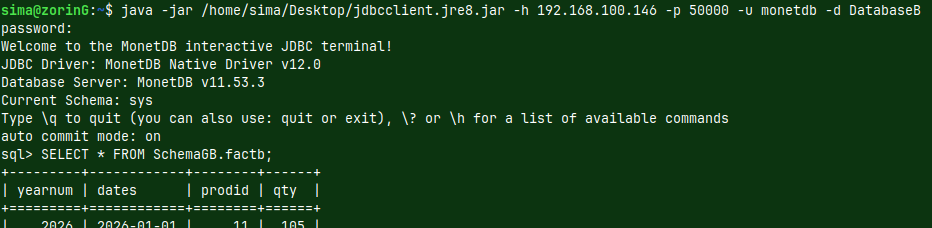
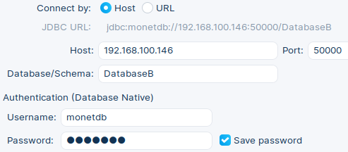
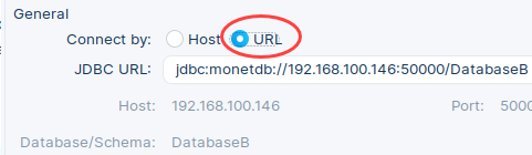
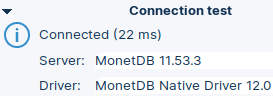
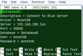
| I will now jump into green server. I explained how to create green server in this blog post "link". I am using this server because that server is set to accept external connections. Green server has IP address "192.168.100.145" and database DatabaseG. | |
I will run this command on the green server, so I am just doing backup locally. msqldump -h 192.168.100.145 -p 50000 -u monetdb -d DatabaseG -o /home/sima/Desktop/DatabaseG_db.sql |  |
I will now run the same command from the "voc" server. This will backup "DatabaseG", from the green server, onto "voc" server. msqldump -h 192.168.100.145 -p 50000 -u monetdb -d DatabaseG -o /home/fffovde/Desktop/DatabaseG_db.sql |  |
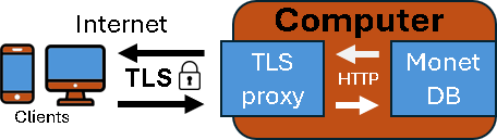
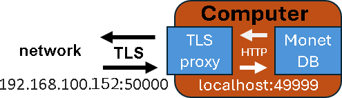
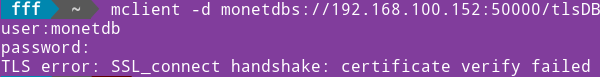
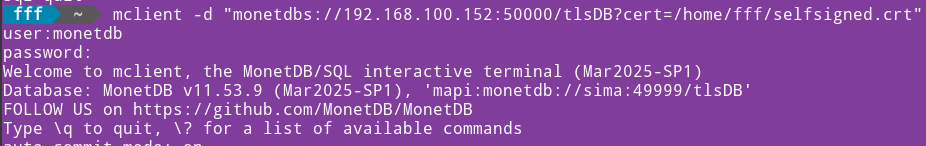
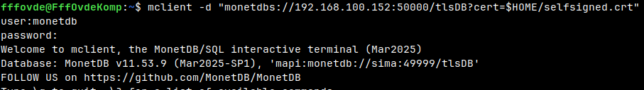
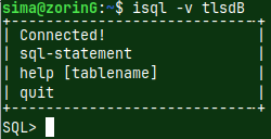
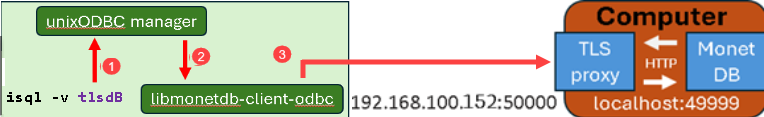
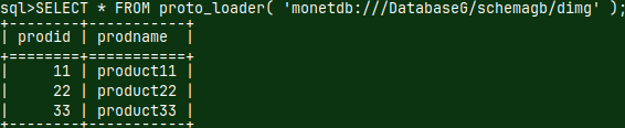
In the previous blogpost "link", I have created purple server, which is protected with TLS. IP address of this server is 192.168.100.152, and its database is "tlsDB". I will now run this command on the "voc" server to backup database from the purple server. msqldump -u monetdb -d 'monetdbs://192.168.100.152:50000/tlsDB?cert=/home/fffovde/selfsigned.crt' -o /home/fffovde/Desktop/tlsDB_db.sql |  |
By providing IP address and the port number, we can backup database locally, or we can pull it from the remote server, even if it is protected with TLS.
Other Msqldump Options
We will run these commands on the "voc" server.
Whichever way we create a backup, at the beginning of the sql file, we will have a welcome message. msqldump -u monetdb -d voc -o /home/fffovde/Desktop/voc_db.sql |  |
We have to add "quiet" switch to avoid that message.msqldump -q -u monetdb -d voc -o /home/fffovde/Desktop/voc_db.sql |  |
If we use "-X" option, we will get message for every step msqldump is doing.msqldump -X -u monetdb -d voc -o /home/fffovde/Desktop/voc_db.sql |  |
| By running this command in the shell, we will get a list of all of the possible options in Msqldump. msqldump -?  We can notice that longer syntax for any option exists, too: msqldump --help | Usage: msqldump [ options ] [ dbname ]-N | --inserts use INSERT INTO statements -q | --quiet don't print welcome message |
Environment Variables
Environment variables are global variables that can be accessed by any process. They are key-value pairs that provide a way for processes to communicate with each other and the operating system.
We can list all the environment variables with "printenv".  | For specific variables we just grep the result of "printenv": printenv | grep home  | If we know the name of variable, then we can read its value with "echo":echo "$HOME" |
My local time is set to Serbian.echo "$LC_TIME" #sr_RSdate # нед, 10. авг 2025. 09:48:22 CEST  | For this session I will set it to English. Set means that we will create or update variable. export LC_TIME=en_US.utf8 date # Sun 10 Aug 2025 09:56:16 AM CEST | With "unset", we will remove variable from the current session. unset LC_TIME |
# export LC_TIME=en_US.utf8 This command will set environment variable permanently if we write it to the file "$HOME/.bashrc". cat /home/fffovde/.bashrc After that, we reload this file with: source ~/.bashrc #tilda is the same as $HOME, or "/home/fffovde" in this case. |  |
DOTMONETDBFILE Environment Variable
If we want to make our Msqldump commands shorter, we can place values for some of the options into file. DOTMONETDBFILE is an environment variable with the path toward that file.
In the temporary folder I already have the file ".monetdb". It has username and password. This is the file we have moved before. I will add IP address and port number of the green server into this file. nano /tmp/.monetdb I will set my DOTMONETDBFILE environment variable to this file. This will be valid for one session. export DOTMONETDBFILE=/tmp/.monetdb | user=monetdb password=monetdb host=192.168.100.145 port=50000 |
Now we can use Msqldump, to backup DatabaseG from the green computer, without providing all the credentials inside of the command. All the credentials are already stored in the ".monetdb" file.msqldump -d DatabaseG -o /home/fffovde/Desktop/DatabaseG_db.sql |  |
Default Folders for .monetdb File
DOTMONETDBFILE is only used if we want to keep ".monetdb" in non-standard folder. For standard folders, we don't need DOTMONETDBFILE. We just have to place the file into one of the standard folders, and this is how we used ".monetdb" file before the talk about environment variables. | 1) Current directory. 2) Path inside of the $XDG_CONFIG_HOME variable (if exists). 3) $HOME directory. |
Msqldump will first look for a ".monetdb" in the current directory, then in $XDG_CONFIG_HOME, and at the end in the $HOME ( /home/fffovde ).
I will move ".monetdb" file into "/home/fffovde", and I will disable DOTMONETDBFILE:mv /tmp/.monetdb /home/fffovde/ unset DOTMONETDBFILE | |
If we now try to run Msqldump, it will read ".monetdb" from the current folder and will work. msqldump -d DatabaseG -o /home/fffovde/Desktop/DatabaseG_db.sql |  |
Ignoring Default Folders
If we set DOTMONETDBFILE to empty string, Msqldump will ignore all of the configuration files, and will always ask for credentials.
# export DOTMONETDBFILE=""From here you can download "voc" database sql dump file (schema file).