Excel

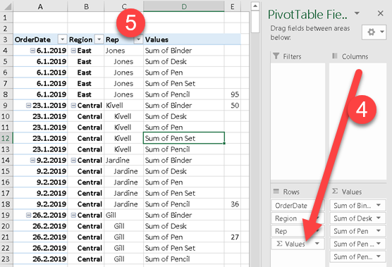
Parts of Pivot Style

This is the standard dialog for changing the pivot table style. Below we will list the elements of this style that can be changed, with the corresponding images.

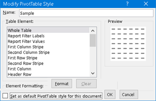
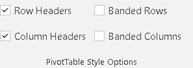
Some of these changes require that the appropriate Pivot Style Options are enabled.

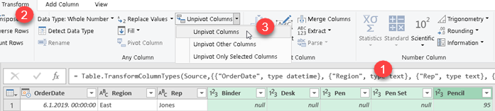
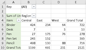
"Whole Table" will affect all parts of the pivot table, including filters.

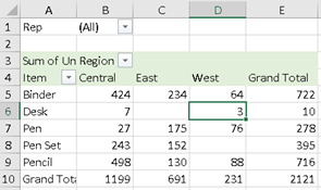
"Report Filter Labels" and "Report Filter Values" will only affect the filter section.

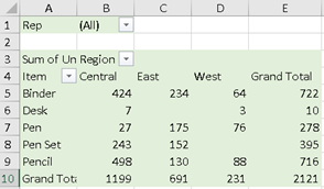
"First and Second Column Stripe", "First and Second Row Stripe", will alternately color columns and rows. If we specify both rows and columns, they will overlap, but the rows will have priority. It is possible for the same color to repeat multiple columns/rows. For example, we can have two green and then two orange columns and so on alternately.

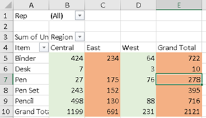
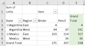
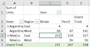
The "First Column" and "Header Row" can also overlap, in the corner cell. Here too, the color given to the row will take precedence.

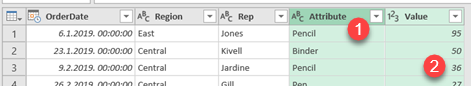
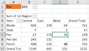
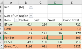
"The First Header Cell" will color the top left cell in the pivot body. The name of the measure used is usually written there.

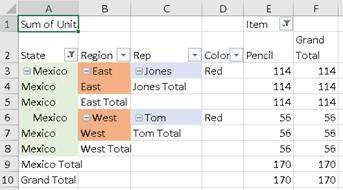
"Subtotal Column" and "Subtotal Row" will color the subtotals by columns and rows. There are "Subtotal Column 1,2,3" and "Subtotal Row 1,2,3", so the first three levels of subtotals can have their own colors.

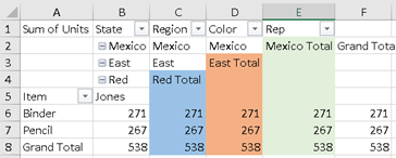
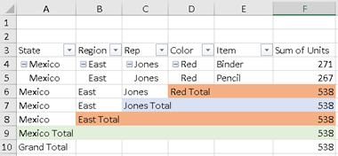
If we turn on the "Blank Row" option then we will have an empty line after each subtotal. The "Blank Row" part of pivot style will color all rows below the first blank row.

"Column Subheading" and "Row Subheading" will color the row and column headers. There are "Column Subheading 1,2,3" as well as "Row Subheading 1,2,3" so we can have up to three colors for different levels of headers.

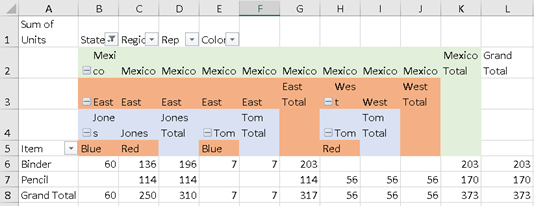
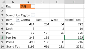
For totals we have the opportunity to design "Grand Total Column" and "Grand Total Row".

Sample Excel file can be downloaded here:

Volatile, Reference, Case Sensitive Functions

Volatile functions

Volatile functions are recalculated each time any cell in the spreadsheet is changed. Some other actions can also cause recalculation, such as renaming sheets, inserting columns, deleting rows, etc. Any formula that contains a volatile function will also become volatile. Any cell that depends on a cell that contains volatile function will also become volatile. Too many cells that contain a volatile function in a spreadsheet will significantly slow down that spreadsheet.

Volatile functions are RAND, RANDBETWEEN, RANDARRAY, NOW, TODAY, OFFSET, INDIRECT. INFO and CELL functions can be volatile depending on which arguments they use.

UDF functions can become volatile if the statement "Application.Volatile" is placed in front of them. The function below is nonvolatile.

Function UnVolatileFunction()
UnVolatileFunction = ActiveCell.Offset(-2, 0).Value + ActiveCell.Offset(-1, 0).Value
End Function

In contrast, this function is volatile because it contains an "Application.Volatile" statement..

Function VolatileFunction()
Application.Volatile
VolatileFunction = ActiveCell.Offset(-2, 0).Value + ActiveCell.Offset(-1, 0).Value
End Function

Excel Functions That Return References

Excel functions that return references are OFFSET, INDEX, XLOOKUP, CHOOSE, SWITCH, IF, IFS, INDIRECT. This means that the result of the function is neither a scalar nor an array. The result is the address of the range in the table.

Although the reference refers to multiple cells, Excel 365 or 2021 can directly display the result of these functions as a spill (1). In older versions of Excel, it was necessary to convert these functions into array functions with Ctrl + Shift + Enter in order to display their result directly (2). If a given range contains only one cell, all versions of Excel will return the contents of that cell (3). If a range contains more than one cell, it has always been possible to wrap that range in an aggregate function that will result in a scalar that can be displayed in a spreadsheet (4).

Case Sensitive Excel Functions

In Excel, there are three functions that are case sensitive. Those are EXACT, FIND and SUBSTITUTE. There are also XLOOKUP and XMATCH functions that have arguments that can be used to control whether the functions are case sensitive. Those functions are available in Excel 365 and 2021.

Direct comparison of A1 and B1 cells will return TRUE (1), but if we use EXACT function, result will be FALSE (2).

How to unpivot Excel tables

Unpivot by using pivot table

This technique is only useful for unpivoting tables with smaller number of columns. Power Query is preferable for larger tables.

We have a table with a pivoted column of office products. We want to unpivot that column.

All we have to do is to create a normal Pivot table. In this pivot table all unchanged columns should be placed into Rows section (1). All other columns, that should be unpivoted, should be placed in Values section (2). Notice that in Columns section we have a special column "∑ Values" (3), that Excel created itself.

Now drag that special "∑ Values" column into Rows section (4). We will immediately get unpivoted table (5). This table asks for some maintenance so is best to make a copy of it in spreadsheet and then fix its header, and filter rows with no values.

This approach could will not be optimal when there are many columns that should be unpivoted. In that case we have to move all those columns into Values section manually. This could be tedious. In that case it is much easier to use Power Query unpivot tool.

Unpivot by using Power Query

Get your unpivoted table into Power Query. Select all columns that should be unpivoted (1). In Transform tab (2) find command "Unpivot Columns" (3). This command will do all the work. Notice that we also have command "Unpivot Other Columns" (3). This allow us to select only columns that shouldn't be unpivoted, and then all the other columns will be unpivoted. When we have really big number of columns to unpivot, this command make it even more easier to accomplish our task.

At the end we get unpivoted table. Again, we have to fix column names (1). Rows without vales will be automatically filtered (2).

Excel sample file:

Instructional video: